CCL19-expressing FRC subsets in coronavirus-vector based immunotherapy
Chrysa Papadopoulou
Last updated: 2024-11-05
Checks: 7 0
Knit directory: CCL19_FRCs_lung_cancer/
This reproducible R Markdown analysis was created with workflowr (version 1.7.1). The Checks tab describes the reproducibility checks that were applied when the results were created. The Past versions tab lists the development history.
Great! Since the R Markdown file has been committed to the Git repository, you know the exact version of the code that produced these results.
Great job! The global environment was empty. Objects defined in the global environment can affect the analysis in your R Markdown file in unknown ways. For reproduciblity it’s best to always run the code in an empty environment.
The command set.seed(20240808) was run prior to running
the code in the R Markdown file. Setting a seed ensures that any results
that rely on randomness, e.g. subsampling or permutations, are
reproducible.
Great job! Recording the operating system, R version, and package versions is critical for reproducibility.
Nice! There were no cached chunks for this analysis, so you can be confident that you successfully produced the results during this run.
Great job! Using relative paths to the files within your workflowr project makes it easier to run your code on other machines.
Great! You are using Git for version control. Tracking code development and connecting the code version to the results is critical for reproducibility.
The results in this page were generated with repository version 60ad221. See the Past versions tab to see a history of the changes made to the R Markdown and HTML files.
Note that you need to be careful to ensure that all relevant files for
the analysis have been committed to Git prior to generating the results
(you can use wflow_publish or
wflow_git_commit). workflowr only checks the R Markdown
file, but you know if there are other scripts or data files that it
depends on. Below is the status of the Git repository when the results
were generated:
Ignored files:
    Ignored:    .DS_Store
    Ignored:    analysis/.DS_Store
    Ignored:    data/Final_submission/
    Ignored:    data/Human/
    Ignored:    data/Mouse/
    Ignored:    data/Public/
    Ignored:    output/GSEA_AdvFB_SULF1/
    Ignored:    output/GSEA_AdvFB_TLS/
    Ignored:    output/GSEA_CCR7_T/
    Ignored:    output/GSEA_CD8_T/
    Ignored:    output/GSEA_CYCL_T/
    Ignored:    output/GSEA_EXH_T/
    Ignored:    output/GSEA_SMC_PRC/

Untracked files:
    Untracked:  README.html
    Untracked:  analysis/.h5seurat
    Untracked:  analysis/Compare_tumors.Rmd
    Untracked:  analysis/NSCLC_PDAC_CAFs.Rmd
    Untracked:  analysis/Seurat_to_SCE.Rmd
    Untracked:  analysis/compression.Rmd
    Untracked:  analysis/index_hidden.Rmd

Unstaged changes:
    Modified:   analysis/index.Rmd
Note that any generated files, e.g. HTML, png, CSS, etc., are not included in this status report because it is ok for generated content to have uncommitted changes.
These are the previous versions of the repository in which changes were
made to the R Markdown (analysis/Mouse_mCOV.Rmd) and HTML
(docs/Mouse_mCOV.html) files. If you’ve configured a remote
Git repository (see ?wflow_git_remote), click on the
hyperlinks in the table below to view the files as they were in that
past version.
| File | Version | Author | Date | Message |
|---|---|---|---|---|
| Rmd | 60ad221 | Pchryssa | 2024-11-05 | Correct figure ordering |
| html | f1b6d9b | Pchryssa | 2024-09-23 | Build site. |
| Rmd | 41217c2 | Pchryssa | 2024-09-23 | Modify figure order |
| html | 3172731 | Pchryssa | 2024-08-21 | Build site. |
| Rmd | 09ceaf1 | Pchryssa | 2024-08-21 | mCOV add thresh |
| html | e852545 | Pchryssa | 2024-08-21 | Build site. |
| Rmd | 512f20d | Pchryssa | 2024-08-21 | Mouse mCOV |
Load packages
suppressPackageStartupMessages({
  library(here)
  library(purrr)
  library(dplyr)
  library(stringr)
  library(patchwork)
  library(Seurat)
  library(Matrix)
  library(dittoSeq)
  library(gridExtra)
  library(gsubfn)
  library(ggsci)
  library(slingshot)
  library(tradeSeq)
  library(mgcv)
})
Set directory
basedir <- here()Read CCL19-EYFP⁺ mCOV-FIt31-g33 cell data
CCL19_EYFP_mCOV <- readRDS(paste0(basedir,"/data/Mouse/mCOV.rds"))Define color palette
cols <- c("#C77CFF","#F8766D","#00BA38","#B79F00","#FF64B0","#00BFC4","#00B4F0","#7CAE00")
names(cols) <-c(paste0("Smoc1", expression("\u207A "), "AdvFB"),paste0("Cd34", expression("\u207A "), "AdvFB"),paste0("Npnt", expression("\u207A "), "AlvFB"),paste0("Hhip", expression("\u207A "), "AdvFB"),paste0("Sulf1", expression("\u207A "), "TRC"),paste0("Rgs5", expression("\u207A "), "PRC"),"SMC/PC","TLS TRC")
CCL19-EYFP⁺ mCOV-FIt31-g33 cells
Umap colored per celltype (Supplementary Figure 5C)
DimPlot(CCL19_EYFP_mCOV, reduction = "umap", group.by = "annot", cols=cols)+
  theme_bw() +
  theme(axis.text = element_blank(), axis.ticks = element_blank(),
        panel.grid.minor = element_blank(),
        panel.grid.major = element_blank()) +
  xlab("UMAP1") +
  ylab("UMAP2") + ggtitle(paste0("Ccl19-EYFP", "\U207A ", "cells (mCOV-FIt31-g33 cells)"))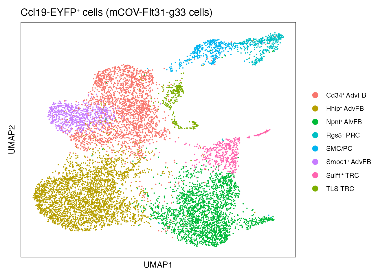
| Version | Author | Date |
|---|---|---|
| 80d46cf | Pchryssa | 2024-08-26 |
Dotplot (Figure 6F)
data_conv <-CCL19_EYFP_mCOV
data_conv <-Remove_ensebl_id(data_conv)

Idents(data_conv) <- data_conv$annot
levels(data_conv)<-levels(data_conv)[order(match(levels(data_conv),c(paste0("Cd34", expression("\u207A "), "AdvFB"),paste0("Smoc1", expression("\u207A "), "AdvFB"),paste0("Hhip", expression("\u207A "), "AdvFB"),paste0("Npnt", expression("\u207A "), "AlvFB"),paste0("Sulf1", expression("\u207A "), "TRC"),paste0("Rgs5", expression("\u207A "), "PRC"),"SMC/PC","TLS TRC")))]
data_conv$annot <- factor(as.character(data_conv@active.ident), levels = rev(c(paste0("Cd34", expression("\u207A "), "AdvFB"),paste0("Smoc1", expression("\u207A "), "AdvFB"), paste0("Hhip", expression("\u207A "), "AdvFB"),paste0("Npnt", expression("\u207A "), "AlvFB"),paste0("Sulf1", expression("\u207A "), "TRC"),paste0("Rgs5", expression("\u207A "), "PRC"),"SMC/PC","TLS TRC")))

gene_list <-c("Cd34","Pdpn","Hhip","Sulf1","Ccl11","Cxcl9","Tnc","Pdgfrb","Notch3","Rgs5","Acta2","Des","Myh11","Il33","Ccl19","Ccl21a","Cxcl13","Clu")

gg <-DotPlot(data_conv, features = gene_list, group.by = "annot", scale = TRUE, cols = c("lightgrey", "#C51B7D"),
             scale.min = 0, scale.max = 100,col.min = 0, col.max = 8 , dot.scale = 4) + xlab(" ") + ylab(" ")

gg + theme(axis.text.x = element_text(angle = 45,hjust = 1))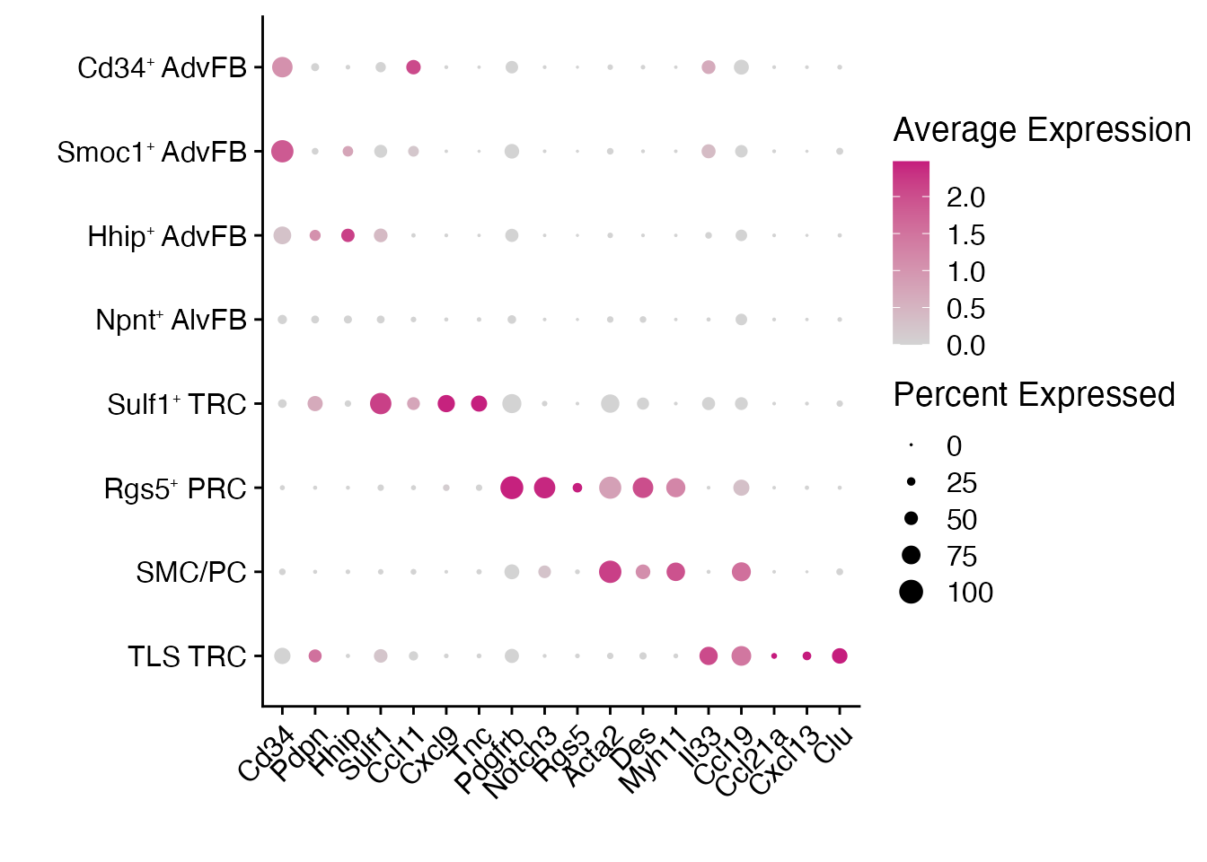
| Version | Author | Date |
|---|---|---|
| 80d46cf | Pchryssa | 2024-08-26 |
Differentiation trajectories on CCL19-EYFP⁺ mCOV-FIt31-g33 cells based on Slingshot algorithm (Figure 6G)
Annotation from RNA_snn_res.0.25 to perform trajectory analysis
#Set color palette
palet_new <- c("#C77CFF","#F8766D","#00BA38","#B79F00","#FF64B0","#00BFC4","#00B4F0","#7CAE00")
names(palet_new) <-c(2,1,4,3,5,6,7,8)

CCL19_EYFP_mCOV$annot_numeric <- CCL19_EYFP_mCOV$annot
CCL19_EYFP_mCOV$annot_numeric[which(CCL19_EYFP_mCOV$annot == paste0("Cd34", expression("\u207A "), "AdvFB"))] <- 1
CCL19_EYFP_mCOV$annot_numeric[which(CCL19_EYFP_mCOV$annot == paste0("Smoc1", expression("\u207A "), "AdvFB"))] <- 2
CCL19_EYFP_mCOV$annot_numeric[which(CCL19_EYFP_mCOV$annot == paste0("Hhip", expression("\u207A "), "AdvFB"))] <- 3
CCL19_EYFP_mCOV$annot_numeric[which(CCL19_EYFP_mCOV$annot == paste0("Npnt", expression("\u207A "), "AlvFB"))] <- 4
CCL19_EYFP_mCOV$annot_numeric[which(CCL19_EYFP_mCOV$annot == paste0("Sulf1", expression("\u207A "), "TRC"))] <- 5
CCL19_EYFP_mCOV$annot_numeric[which(CCL19_EYFP_mCOV$annot == paste0("Rgs5", expression("\u207A "), "PRC"))] <- 6
CCL19_EYFP_mCOV$annot_numeric[which(CCL19_EYFP_mCOV$annot == "SMC/PC")] <- 7
CCL19_EYFP_mCOV$annot_numeric[which(CCL19_EYFP_mCOV$annot == "TLS TRC")] <- 8

DimPlot(CCL19_EYFP_mCOV, reduction = "umap", group.by = "annot_numeric", cols = palet_new)+
  theme_bw() +
  theme(axis.text = element_blank(), axis.ticks = element_blank(),
        panel.grid.minor = element_blank(),
        panel.grid.major = element_blank()) +
  xlab("UMAP1") +
  ylab("UMAP2") + ggtitle("New annotation")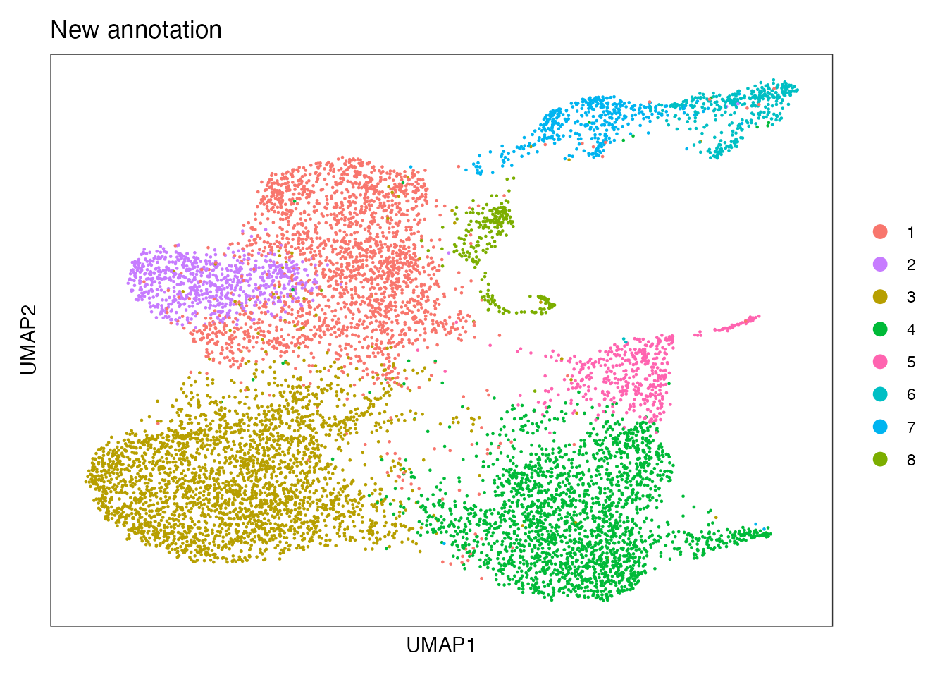
| Version | Author | Date |
|---|---|---|
| 80d46cf | Pchryssa | 2024-08-26 |
Differentiation trajectories for Sulf1⁺ TRC, TLS TRC and Rgs5⁺ PRC
#Calculation of CCL19-EYFP`r knitr::asis_output("\U207A")` mCOV-FIt31-g33 cell differentiation trajectories
clustering <- CCL19_EYFP_mCOV@meta.data$annot_numeric
dimred <- CCL19_EYFP_mCOV@reductions$umap@cell.embeddings

# Slingshot for TRC (Sulf1, TLS)
pto_TRC <- slingshot(dimred, clustering, start.clus = '2', end.clus = '8', reducedDim = 'umap',extend="n",stretch=0.07,thresh=0.05)
pto_TRC <- as.SlingshotDataSet(pto_TRC)

# Slingshot for PRC
pto_PRC <- slingshot(dimred, clustering, start.clus = '7', end.clus = '6' ,reducedDim = 'umap',extend="n",stretch=0.07,thresh=0.05)
pto_PRC <- as.SlingshotDataSet(pto_PRC)

plot(dimred, col = palet_new[clustering], asp = 1, pch = 16)
lines(pto_PRC@curves$Lineage3, lwd = 3, col = 'magenta')
lines(pto_TRC@curves$Lineage3, lwd = 3, col = 'gold')
lines(pto_TRC@curves$Lineage1, lwd = 3, col = 'black')
legend("bottomright", legend = c("T3"), col = c('gold'), lty = 1, lwd = 2.5, cex = 1.1)
legend("topright", legend = names(cols), col = cols, pch = 2, pt.cex = 1, cex = 0.8)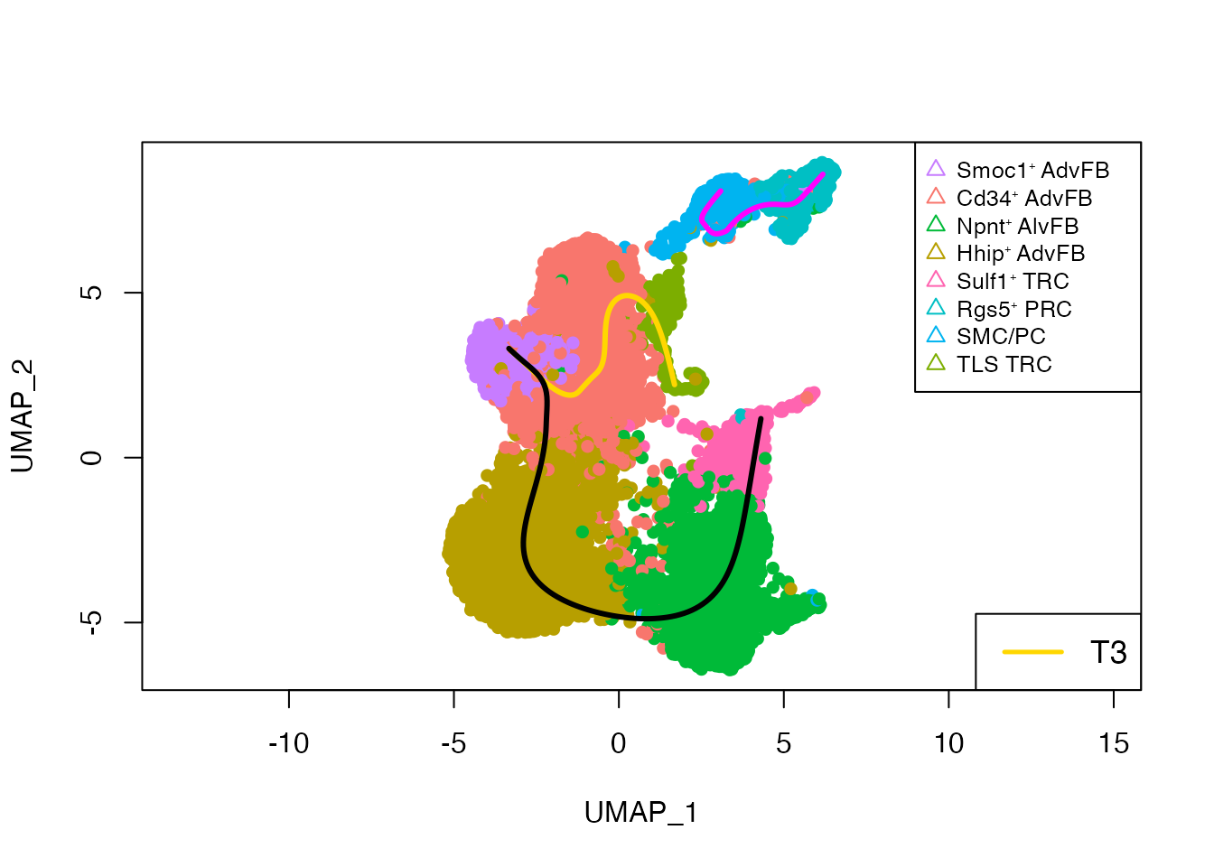
| Version | Author | Date |
|---|---|---|
| 80d46cf | Pchryssa | 2024-08-26 |
Combine gene signatures in T3 differentiation trajectory (Figure 6H)
counts <- CCL19_EYFP_mCOV@assays$RNA@counts

CCL19_EYFP_mCOV <- FindVariableFeatures(CCL19_EYFP_mCOV, selection.method = "vst", nfeatures = 1000)

new_counts <-counts[rownames(counts) %in% CCL19_EYFP_mCOV@assays$RNA@var.features,]
sds <- as.SlingshotDataSet(pto_TRC)
pseudotime <- slingPseudotime(pto_TRC, na = FALSE)
cellWeights <- slingCurveWeights(pto_TRC)

BPPARAM <- BiocParallel::bpparam()
BPPARAM$workers <- 4 # use 2 cores
control <- gam.control()
control$maxit <- 1000
set.seed(3)
sce <- fitGAM(counts = new_counts, pseudotime = pseudotime, cellWeights = cellWeights,
nknots = 6, verbose = TRUE,parallel=TRUE, BPPARAM = BPPARAM, sds = sds,control = control)Save sce object
#saveRDS(sce, paste0(basedir,"/data/Mouse/Trajectory_fitGAM_T3_1000.rds"))Read sce object
We provide the sce object because the fitGAM commnand took time to run
sce <- readRDS(paste0(basedir,"/data/Mouse/Trajectory_fitGAM_T3_1000.rds"))We focus on genes whose expression changes across the T3 trajectory in the pseudotime. In particular, on those genes that are upregulated in TLS TRC. We use the startVsEndTest statistical test.
Gene expression changes in T3 trajectory
pseudotime_start_end_association <- startVsEndTest(sce) Calculate log-transformed counts and fitted values for a particular gene across the T3 lineage
data_Ccl21a <-plotSmoothers1(sce, counts, gene = "ENSMUSG00000094686.Ccl21a", lineagesToPlot = c(3))
data_Srgn <-plotSmoothers1(sce, counts, gene = "ENSMUSG00000020077.Srgn", lineagesToPlot = c(3))
data_Il33 <-plotSmoothers1(sce, counts, gene = "ENSMUSG00000024810.Il33", lineagesToPlot = c(3))
data_Cxcl12 <-plotSmoothers1(sce, counts, gene = "ENSMUSG00000061353.Cxcl12", lineagesToPlot = c(3))
data_Ccl19 <-plotSmoothers1(sce, counts, gene = "ENSMUSG00000071005.Ccl19", lineagesToPlot = c(3))

data_Ccl21a$gene <- "Ccl21a"
data_Srgn$gene <-"Srgn"
data_Il33$gene <-"Il33"
data_Cxcl12$gene <-"Cxcl12"
data_Ccl19$gene <-"Ccl19"
Plot gene curves
cols_pal <- c("orange","#00B0F6","#00BB4E","#C09B00", "#FF6A98")
names(cols_pal) <-c("Ccl19","Il33","Cxcl12","Ccl21a","Srgn")

visual12 <- rbind(data_Ccl21a,data_Srgn,data_Il33,data_Cxcl12,data_Ccl19)
end_val <-round(max(visual12$time)) + 1
end_y_axis <-round(max(log1p(visual12$gene_count)))

ggplot(visual12, aes(x=time, y=log1p(gene_count), group=gene, col = gene, fill=gene)) +
  labs(x = "Pseudotime (T3)", y = "Log(expression + 1)") +
      geom_line(lwd = 2) +
  scale_y_continuous(expand = expansion(c(0,0)), limits = c(0.0, end_y_axis),breaks = c(0,1,2,3,4,end_y_axis)) +
  scale_x_continuous(limits = c(0.0, end_val + 0.5), expand = expansion(c(0,0)), breaks = c(0,5,end_val)) +
 theme(aspect.ratio=1.3, axis.text.y = element_text(angle = 0,colour = "black")) +
  theme(axis.line = element_line(colour = "black"),
panel.grid.major = element_blank(),
panel.grid.minor = element_blank(),
panel.border = element_blank(),
panel.background = element_blank(),
legend.title = element_blank(),axis.text.x = element_text(angle = 0, vjust = 0.5,colour = "black")) +
  scale_color_manual(values = cols_pal)+
  ggtitle(paste0("Cd34", "\U207A ", "AdvFB >> TLS TRC (T3)"))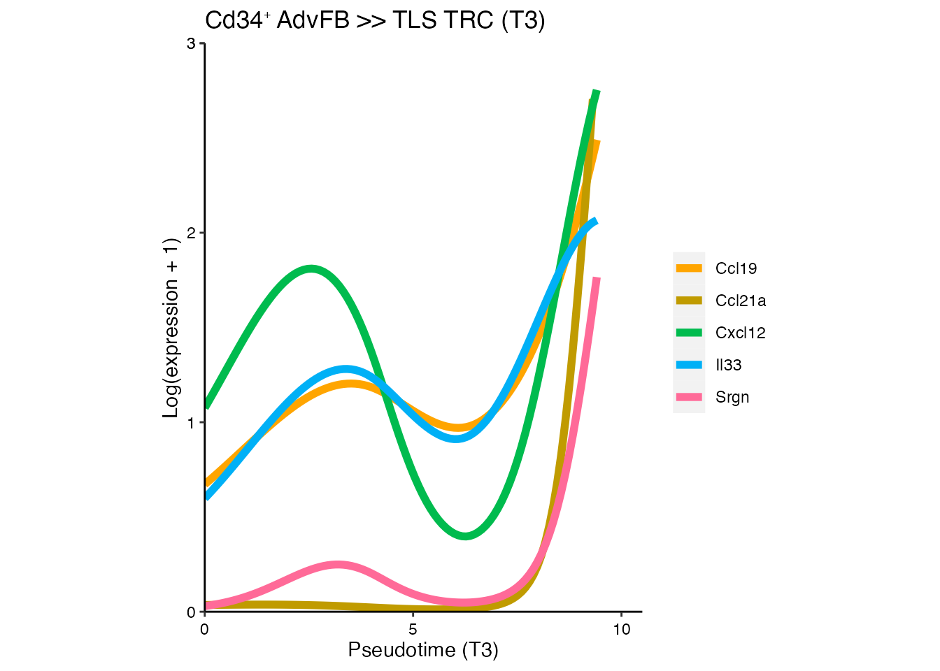
| Version | Author | Date |
|---|---|---|
| 80d46cf | Pchryssa | 2024-08-26 |
Multidimensional scaling (MDS) plot
Multidimensional scaling (MDS) visualizes the level of similarity of variables in a data set. MDS recognizes the structure of the dataset in 2D, as it maintains the pairwise distances between data points.
Read CCL19-EYFP⁺ cell data from naïve lungs and excised LLC-gp33 tumors on day 23
CCL19_EYFP <- readRDS(paste0(basedir,"/data/Mouse/CCL19_EYFP_nonmCOV.rds"))Merge CCL19-EYFP⁺ cells from mCOV-FIt31-g33 and non immunization
data_merge <- merge(CCL19_EYFP, y = c(CCL19_EYFP_mCOV),
             add.cell.ids = c("CCL19_EYFP","CCL19_EYFP_mCOV"),
             project = "merge_no_mcov_mcov")

#Preprocessing
resolution <- c(0.1, 0.25, 0.4, 0.6,0.8, 1.)
data_merge  <- preprocessing(data_merge,resolution)
Modularity Optimizer version 1.3.0 by Ludo Waltman and Nees Jan van Eck
Number of nodes: 15462
Number of edges: 511917
Running Louvain algorithm...
Maximum modularity in 10 random starts: 0.9547
Number of communities: 5
Elapsed time: 1 seconds
Modularity Optimizer version 1.3.0 by Ludo Waltman and Nees Jan van Eck
Number of nodes: 15462
Number of edges: 511917
Running Louvain algorithm...
Maximum modularity in 10 random starts: 0.9218
Number of communities: 9
Elapsed time: 1 seconds
Modularity Optimizer version 1.3.0 by Ludo Waltman and Nees Jan van Eck
Number of nodes: 15462
Number of edges: 511917
Running Louvain algorithm...
Maximum modularity in 10 random starts: 0.8969
Number of communities: 11
Elapsed time: 1 seconds
Modularity Optimizer version 1.3.0 by Ludo Waltman and Nees Jan van Eck
Number of nodes: 15462
Number of edges: 511917
Running Louvain algorithm...
Maximum modularity in 10 random starts: 0.8737
Number of communities: 15
Elapsed time: 1 seconds
Modularity Optimizer version 1.3.0 by Ludo Waltman and Nees Jan van Eck
Number of nodes: 15462
Number of edges: 511917
Running Louvain algorithm...
Maximum modularity in 10 random starts: 0.8545
Number of communities: 16
Elapsed time: 1 seconds
Modularity Optimizer version 1.3.0 by Ludo Waltman and Nees Jan van Eck
Number of nodes: 15462
Number of edges: 511917
Running Louvain algorithm...
Maximum modularity in 10 random starts: 0.8371
Number of communities: 16
Elapsed time: 1 secondsIntegrate data to correct for batch effects due to different condition (naive vs mCOV-FIt31-g33) via seurat
Step 1
#Split object by Patient as we see batch effects coming from different patients
obj.list <-SplitObject(data_merge, split.by = 'condition')
#For each object in list we see to run normalization and identify highly variable features
for (i in 1:length(obj.list)){
  #Normalization
  obj.list[[i]] <- NormalizeData(obj.list[[i]], normalization.method = "LogNormalize", scale.factor = 10000)
  #Find high variable genes
  obj.list[[i]] <- FindVariableFeatures(obj.list[[i]], selection.method = "vst", nfeatures = 2000)#The purpose of this is to id
}
Step 2
#select features that are repeatedly variable across datasets for integration
features <- SelectIntegrationFeatures(object.list = obj.list)
#Find anchors to integrate the data across different patients (Canonical correlation analysis)
anchors <- FindIntegrationAnchors(object.list = obj.list, anchor.features = features)
# this command creates an 'integrated' data assay
seurat_integrated <- IntegrateData(anchorset = anchors)
Step 3
# We run a single integrated analysis on all cells!
DefaultAssay(seurat_integrated) <- "integrated"

# Run the standard workflow for visualization and clustering
seurat_integrated <- ScaleData(seurat_integrated, verbose = FALSE)
seurat_integrated <- RunPCA(object = seurat_integrated, npcs = 30, verbose = FALSE,seed.use = 8734)
seurat_integrated <- RunTSNE(object = seurat_integrated, reduction = "pca", dims = 1:20, seed.use = 8734)
seurat_integrated<- RunUMAP(object = seurat_integrated, reduction = "pca", dims = 1:20, seed.use = 8734)
 seurat_integrated <- FindNeighbors(object = seurat_integrated, reduction = "pca", dims = 1:20, seed.use = 8734)
#Clustering
resolution <- c(0.1, 0.25, 0.4, 0.6,0.8, 1.)
for(k in 1:length(resolution)){
  seurat_integrated <- FindClusters(object = seurat_integrated, resolution = resolution[k], random.seed = 8734)
}
Modularity Optimizer version 1.3.0 by Ludo Waltman and Nees Jan van Eck
Number of nodes: 15462
Number of edges: 525485
Running Louvain algorithm...
Maximum modularity in 10 random starts: 0.9570
Number of communities: 5
Elapsed time: 1 seconds
Modularity Optimizer version 1.3.0 by Ludo Waltman and Nees Jan van Eck
Number of nodes: 15462
Number of edges: 525485
Running Louvain algorithm...
Maximum modularity in 10 random starts: 0.9236
Number of communities: 8
Elapsed time: 1 seconds
Modularity Optimizer version 1.3.0 by Ludo Waltman and Nees Jan van Eck
Number of nodes: 15462
Number of edges: 525485
Running Louvain algorithm...
Maximum modularity in 10 random starts: 0.8964
Number of communities: 11
Elapsed time: 1 seconds
Modularity Optimizer version 1.3.0 by Ludo Waltman and Nees Jan van Eck
Number of nodes: 15462
Number of edges: 525485
Running Louvain algorithm...
Maximum modularity in 10 random starts: 0.8676
Number of communities: 14
Elapsed time: 1 seconds
Modularity Optimizer version 1.3.0 by Ludo Waltman and Nees Jan van Eck
Number of nodes: 15462
Number of edges: 525485
Running Louvain algorithm...
Maximum modularity in 10 random starts: 0.8463
Number of communities: 16
Elapsed time: 1 seconds
Modularity Optimizer version 1.3.0 by Ludo Waltman and Nees Jan van Eck
Number of nodes: 15462
Number of edges: 525485
Running Louvain algorithm...
Maximum modularity in 10 random starts: 0.8299
Number of communities: 18
Elapsed time: 1 secondsBatch effects based on condition are corrected
Color per condition
DimPlot(seurat_integrated, reduction = "umap", group.by = "condition")+
  theme_bw() +
  theme(axis.text = element_blank(), axis.ticks = element_blank(),
        panel.grid.major = element_blank(),
        panel.grid.minor = element_blank()) +
  xlab("UMAP1") +
ylab("UMAP2") 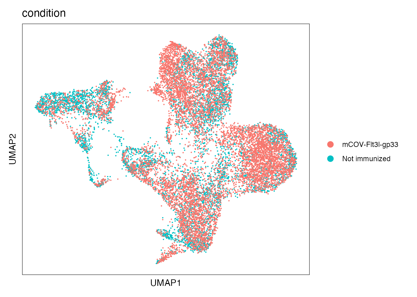
| Version | Author | Date |
|---|---|---|
| 80d46cf | Pchryssa | 2024-08-26 |
Existing cell type annotation
DimPlot(seurat_integrated, reduction = "umap", group.by = "annot")+
  theme_bw() +
  theme(axis.text = element_blank(), axis.ticks = element_blank(),
        panel.grid.major = element_blank(),
        panel.grid.minor = element_blank()) +
  xlab("UMAP1") +
ylab("UMAP2") 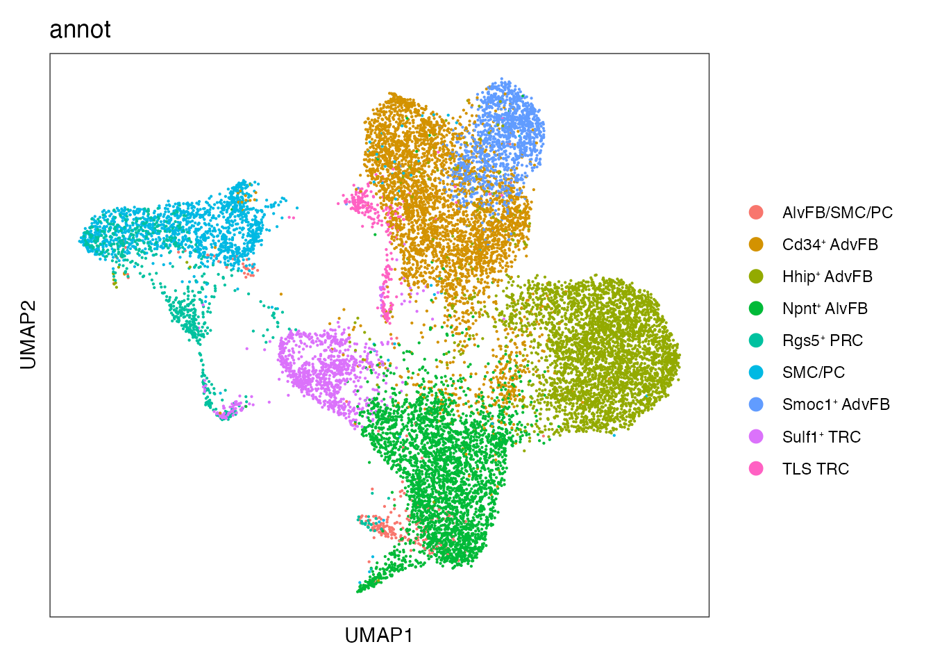
| Version | Author | Date |
|---|---|---|
| 80d46cf | Pchryssa | 2024-08-26 |
Plot gene signatures
DefaultAssay(seurat_integrated)<- "RNA"

genes <- c("NPNT","HHIP","CD34","ACTA2","SULF1","CLU","CCL21A","CCL19","IL33","SMOC1","CXCL13","RGS5")
genes <-str_to_sentence(genes)

genes <- unlist(lapply(genes, function(x) {
  get_full_gene_name(x,seurat_integrated)
}))
NPNT HHIP CD34 ACTA2
DefaultAssay(seurat_integrated)<- "RNA"

FeaturePlot(seurat_integrated, reduction = "umap",
          features = genes[1:4],
          cols=c("lightgrey", "darkred"),
          order = T )+
theme(legend.position="right", legend.title=element_text(size=5)) 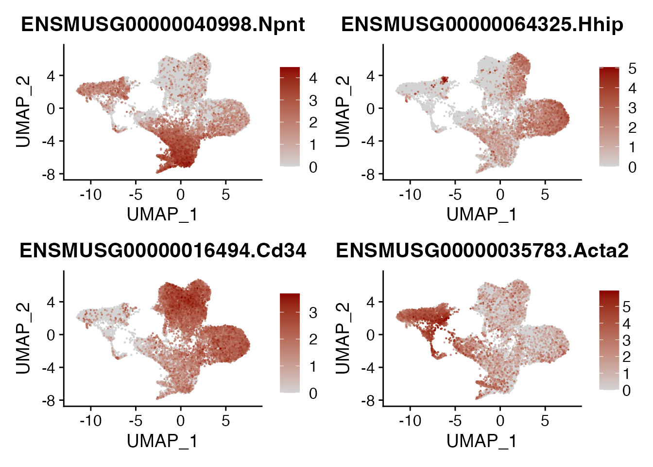
| Version | Author | Date |
|---|---|---|
| 80d46cf | Pchryssa | 2024-08-26 |
SULF1 CLU CCL21A CCL19
DefaultAssay(seurat_integrated)<- "RNA"

FeaturePlot(seurat_integrated, reduction = "umap",
          features = genes[5:8],
          cols=c("lightgrey", "darkred"),
          order = T )+
theme(legend.position="right", legend.title=element_text(size=5)) 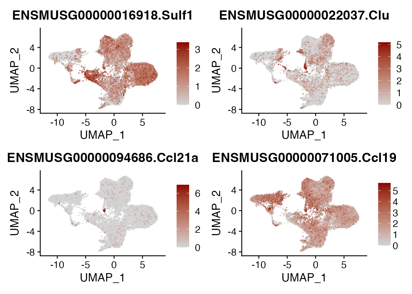
| Version | Author | Date |
|---|---|---|
| 80d46cf | Pchryssa | 2024-08-26 |
IL33 SMOC1 CXCL13 RGS5
DefaultAssay(seurat_integrated)<- "RNA"

FeaturePlot(seurat_integrated, reduction = "umap",
          features = genes[9:12],
          cols=c("lightgrey", "darkred"),
          order = T )+
theme(legend.position="right", legend.title=element_text(size=5)) 
| Version | Author | Date |
|---|---|---|
| 80d46cf | Pchryssa | 2024-08-26 |
Perform new cell type annotation based on the previous gene signatures
DefaultAssay(seurat_integrated) <- "integrated"

seurat_integrated@meta.data$new_annot <--1
seurat_integrated$new_annot[which(seurat_integrated$integrated_snn_res.0.25 == 0)] <- paste0("Cd34", "\u207A ", "AdvFB")

seurat_integrated$new_annot[which(seurat_integrated$integrated_snn_res.0.25 == 1)] <- paste0("Hhip", "\u207A ", "AdvFB")

seurat_integrated$new_annot[which(seurat_integrated$integrated_snn_res.0.25 == 2)] <- paste0("Npnt", "\u207A ", "AlvFB")

seurat_integrated$new_annot[which(seurat_integrated$integrated_snn_res.0.25 == 3)] <- "SMC/PC"

seurat_integrated$new_annot[which(seurat_integrated$integrated_snn_res.0.25 == 4)] <- paste0("Sulf1", "\u207A ", "TRC")

seurat_integrated$new_annot[which(seurat_integrated$integrated_snn_res.0.25 == 5)] <- paste0("Rgs5", "\u207A ", "PRC")

seurat_integrated$new_annot[which(seurat_integrated$integrated_snn_res.0.25 == 6)] <- paste0("Npnt", "\u207A ", "AlvFB")

seurat_integrated$new_annot[which(seurat_integrated$integrated_snn_res.0.25 == 7)] <- paste0("TLS ", "TRC")
Visualize new cell type annotation
DimPlot(seurat_integrated, reduction = "umap", group.by = "new_annot", cols = cols)+
  theme_bw() +
  theme(axis.text = element_blank(), axis.ticks = element_blank(),
        panel.grid.major = element_blank(),
        panel.grid.minor = element_blank()) +
  xlab("UMAP1") +
  ylab("UMAP2") #+ NoLegend()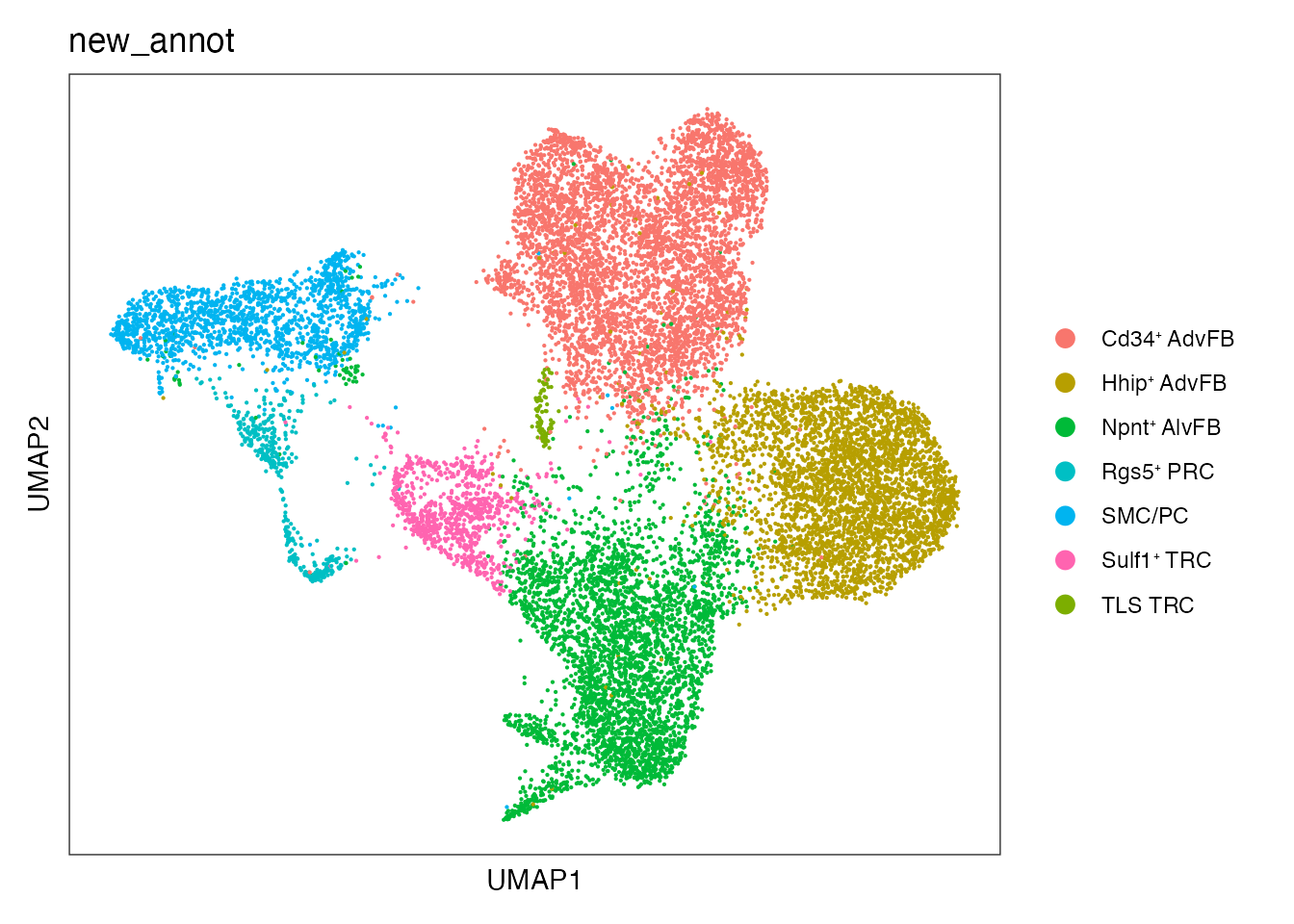
| Version | Author | Date |
|---|---|---|
| 80d46cf | Pchryssa | 2024-08-26 |
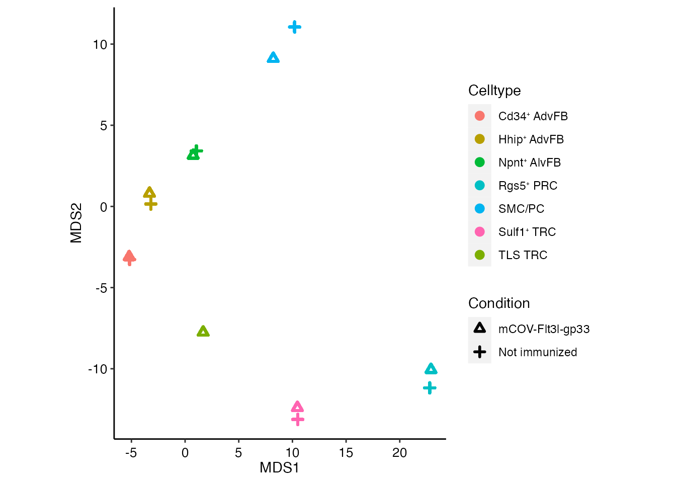
MDS computation
# Before running MDS, we first calculate a distance matrix between all pairs of cells.
# Here we use a simple euclidean distance metric on all genes, using scale.data as input
d <- dist(t(GetAssayData(seurat_integrated, slot = 'scale.data')))
d_mat <-as.matrix(d)
# Run the MDS procedure, k determines the number of dimensions
mds <- cmdscale(d = d, k = 2)
# cmdscale returns the cell embeddings, we first label the columns to ensure downstream consistency
colnames(mds) <- paste0("MDS_", 1:2)
# We will now store this as a custom dimensional reduction called "mds"
seurat_integrated[['mds']] <- CreateDimReducObject(embeddings = mds, key = 'MDS_', assay = DefaultAssay(seurat_integrated))
#saveRDS(seurat_integrated, paste0(basedir,"/data/Mouse/integrated_naive_mcov_mds.rds"))We provide the integrated object with MDS representation as the classical MDS algorithm takes a long time to run.
Read integrated object with MDS representation
seurat_integrated <- readRDS(paste0(basedir,"/data/Mouse/integrated_naive_mcov_mds.rds"))Visualize MDS plot (Figure 6E)
mds_tx_condition = seurat_integrated@reductions$mds@cell.embeddings %>%
as.data.frame() %>% cbind(tx = seurat_integrated@meta.data$condition)

mds_tx_celltype = seurat_integrated@reductions$mds@cell.embeddings %>%
as.data.frame() %>% cbind(tx = seurat_integrated@meta.data$new_annot)

mds_tx_TOTAL <-merge(mds_tx_condition, mds_tx_celltype, by=c("MDS_1", "MDS_2"), all.x=T, all.y=T)
colnames(mds_tx_TOTAL) <-c("MDS_1", "MDS_2", "Condition","Celltype")

mds_tx_TOTAL <- mds_tx_TOTAL %>%
  group_by(Celltype,Condition) %>%
  mutate(count_mds1 = mean(MDS_1)) %>%
  mutate(count_mds2 = mean(MDS_2))

test <-mds_tx_TOTAL %>%
  group_by(Celltype) %>%
  filter(!(Celltype == 'TLS TRC' & Condition == 'Not immunized'))

ggplot(test, aes(x=count_mds1, y=count_mds2, color=Celltype, shape = Condition)) + geom_point(stroke = 1.5) + ylab("MDS2") + xlab("MDS1") +
scale_color_manual(values=cols) + scale_shape_manual(values = c(2, 3)) +
  theme(aspect.ratio = 1.3, axis.line = element_line(colour = "black"),
    panel.grid.major = element_blank(),
    panel.grid.minor = element_blank(),
    panel.border = element_blank(),
    panel.background = element_blank(),
    axis.text.y = element_text(angle = 0, vjust = 0.5,colour = "black",size = 10),
    axis.text.x = element_text(angle = 0, vjust = 0.5,colour = "black",size = 10),

) 
| Version | Author | Date |
|---|---|---|
| 80d46cf | Pchryssa | 2024-08-26 |
Session info
sessionInfo()R version 4.3.1 (2023-06-16)
Platform: aarch64-apple-darwin20 (64-bit)
Running under: macOS Ventura 13.6.9
Matrix products: default
BLAS: /Library/Frameworks/R.framework/Versions/4.3-arm64/Resources/lib/libRblas.0.dylib
LAPACK: /Library/Frameworks/R.framework/Versions/4.3-arm64/Resources/lib/libRlapack.dylib; LAPACK version 3.11.0
locale:
[1] en_US.UTF-8/en_US.UTF-8/en_US.UTF-8/C/en_US.UTF-8/en_US.UTF-8
time zone: Europe/Zurich
tzcode source: internal
attached base packages:
[1] stats4 stats graphics grDevices utils datasets methods
[8] base
other attached packages:
[1] mgcv_1.9-0 nlme_3.1-162
[3] tradeSeq_1.14.0 slingshot_2.8.0
[5] TrajectoryUtils_1.8.0 SingleCellExperiment_1.22.0
[7] SummarizedExperiment_1.30.2 Biobase_2.60.0
[9] GenomicRanges_1.52.0 GenomeInfoDb_1.36.1
[11] IRanges_2.34.1 S4Vectors_0.38.1
[13] BiocGenerics_0.46.0 MatrixGenerics_1.12.3
[15] matrixStats_1.0.0 princurve_2.1.6
[17] ggsci_3.0.0 gsubfn_0.7
[19] proto_1.0.0 gridExtra_2.3
[21] dittoSeq_1.12.1 ggplot2_3.4.2
[23] Matrix_1.6-0 SeuratObject_4.1.3
[25] Seurat_4.3.0.1 patchwork_1.1.2
[27] stringr_1.5.0 dplyr_1.1.2
[29] purrr_1.0.1 here_1.0.1
[31] magrittr_2.0.3 circlize_0.4.15
[33] tidyr_1.3.0 tibble_3.2.1
[35] workflowr_1.7.1
loaded via a namespace (and not attached):
[1] RcppAnnoy_0.0.21 splines_4.3.1
[3] later_1.3.1 bitops_1.0-7
[5] polyclip_1.10-4 lifecycle_1.0.3
[7] tcltk_4.3.1 edgeR_3.42.4
[9] rprojroot_2.0.3 globals_0.16.2
[11] processx_3.8.2 lattice_0.21-8
[13] MASS_7.3-60 limma_3.56.2
[15] plotly_4.10.2 sass_0.4.7
[17] rmarkdown_2.23 jquerylib_0.1.4
[19] yaml_2.3.7 httpuv_1.6.11
[21] sctransform_0.3.5 sp_2.0-0
[23] spatstat.sparse_3.0-2 reticulate_1.36.1
[25] cowplot_1.1.1 pbapply_1.7-2
[27] RColorBrewer_1.1-3 abind_1.4-5
[29] zlibbioc_1.46.0 Rtsne_0.16
[31] RCurl_1.98-1.12 git2r_0.33.0
[33] GenomeInfoDbData_1.2.10 ggrepel_0.9.3
[35] irlba_2.3.5.1 listenv_0.9.0
[37] spatstat.utils_3.1-0 pheatmap_1.0.12
[39] goftest_1.2-3 spatstat.random_3.1-5
[41] fitdistrplus_1.1-11 parallelly_1.36.0
[43] DelayedMatrixStats_1.22.0 leiden_0.4.3
[45] codetools_0.2-19 DelayedArray_0.28.0
[47] tidyselect_1.2.0 shape_1.4.6
[49] farver_2.1.1 viridis_0.6.4
[51] spatstat.explore_3.2-1 jsonlite_1.8.7
[53] ellipsis_0.3.2 progressr_0.13.0
[55] ggridges_0.5.4 survival_3.5-5
[57] systemfonts_1.0.4 tools_4.3.1
[59] ragg_1.2.5 ica_1.0-3
[61] Rcpp_1.0.11 glue_1.6.2
[63] SparseArray_1.2.4 xfun_0.39
[65] withr_2.5.0 fastmap_1.1.1
[67] fansi_1.0.4 callr_3.7.3
[69] digest_0.6.33 R6_2.5.1
[71] mime_0.12 textshaping_0.3.6
[73] colorspace_2.1-0 scattermore_1.2
[75] tensor_1.5 spatstat.data_3.0-1
[77] utf8_1.2.3 generics_0.1.3
[79] data.table_1.14.8 httr_1.4.6
[81] htmlwidgets_1.6.2 S4Arrays_1.2.1
[83] whisker_0.4.1 uwot_0.1.16
[85] pkgconfig_2.0.3 gtable_0.3.3
[87] lmtest_0.9-40 XVector_0.40.0
[89] htmltools_0.5.5 scales_1.2.1
[91] png_0.1-8 knitr_1.43
[93] rstudioapi_0.15.0 reshape2_1.4.4
[95] cachem_1.0.8 zoo_1.8-12
[97] GlobalOptions_0.1.2 KernSmooth_2.23-22
[99] parallel_4.3.1 miniUI_0.1.1.1
[101] pillar_1.9.0 grid_4.3.1
[103] vctrs_0.6.3 RANN_2.6.1
[105] promises_1.2.0.1 xtable_1.8-4
[107] cluster_2.1.4 evaluate_0.21
[109] locfit_1.5-9.8 cli_3.6.1
[111] compiler_4.3.1 rlang_1.1.1
[113] crayon_1.5.2 future.apply_1.11.0
[115] labeling_0.4.2 ps_1.7.5
[117] getPass_0.2-4 plyr_1.8.8
[119] fs_1.6.3 stringi_1.7.12
[121] viridisLite_0.4.2 deldir_1.0-9
[123] BiocParallel_1.34.2 munsell_0.5.0
[125] lazyeval_0.2.2 spatstat.geom_3.2-4
[127] sparseMatrixStats_1.12.2 future_1.33.0
[129] shiny_1.7.4.1 highr_0.10
[131] ROCR_1.0-11 igraph_1.5.0.1
[133] bslib_0.5.0 date()[1] "Tue Nov 5 23:02:34 2024"
sessionInfo()R version 4.3.1 (2023-06-16)
Platform: aarch64-apple-darwin20 (64-bit)
Running under: macOS Ventura 13.6.9
Matrix products: default
BLAS: /Library/Frameworks/R.framework/Versions/4.3-arm64/Resources/lib/libRblas.0.dylib
LAPACK: /Library/Frameworks/R.framework/Versions/4.3-arm64/Resources/lib/libRlapack.dylib; LAPACK version 3.11.0
locale:
[1] en_US.UTF-8/en_US.UTF-8/en_US.UTF-8/C/en_US.UTF-8/en_US.UTF-8
time zone: Europe/Zurich
tzcode source: internal
attached base packages:
[1] stats4 stats graphics grDevices utils datasets methods
[8] base
other attached packages:
[1] mgcv_1.9-0 nlme_3.1-162
[3] tradeSeq_1.14.0 slingshot_2.8.0
[5] TrajectoryUtils_1.8.0 SingleCellExperiment_1.22.0
[7] SummarizedExperiment_1.30.2 Biobase_2.60.0
[9] GenomicRanges_1.52.0 GenomeInfoDb_1.36.1
[11] IRanges_2.34.1 S4Vectors_0.38.1
[13] BiocGenerics_0.46.0 MatrixGenerics_1.12.3
[15] matrixStats_1.0.0 princurve_2.1.6
[17] ggsci_3.0.0 gsubfn_0.7
[19] proto_1.0.0 gridExtra_2.3
[21] dittoSeq_1.12.1 ggplot2_3.4.2
[23] Matrix_1.6-0 SeuratObject_4.1.3
[25] Seurat_4.3.0.1 patchwork_1.1.2
[27] stringr_1.5.0 dplyr_1.1.2
[29] purrr_1.0.1 here_1.0.1
[31] magrittr_2.0.3 circlize_0.4.15
[33] tidyr_1.3.0 tibble_3.2.1
[35] workflowr_1.7.1
loaded via a namespace (and not attached):
[1] RcppAnnoy_0.0.21 splines_4.3.1
[3] later_1.3.1 bitops_1.0-7
[5] polyclip_1.10-4 lifecycle_1.0.3
[7] tcltk_4.3.1 edgeR_3.42.4
[9] rprojroot_2.0.3 globals_0.16.2
[11] processx_3.8.2 lattice_0.21-8
[13] MASS_7.3-60 limma_3.56.2
[15] plotly_4.10.2 sass_0.4.7
[17] rmarkdown_2.23 jquerylib_0.1.4
[19] yaml_2.3.7 httpuv_1.6.11
[21] sctransform_0.3.5 sp_2.0-0
[23] spatstat.sparse_3.0-2 reticulate_1.36.1
[25] cowplot_1.1.1 pbapply_1.7-2
[27] RColorBrewer_1.1-3 abind_1.4-5
[29] zlibbioc_1.46.0 Rtsne_0.16
[31] RCurl_1.98-1.12 git2r_0.33.0
[33] GenomeInfoDbData_1.2.10 ggrepel_0.9.3
[35] irlba_2.3.5.1 listenv_0.9.0
[37] spatstat.utils_3.1-0 pheatmap_1.0.12
[39] goftest_1.2-3 spatstat.random_3.1-5
[41] fitdistrplus_1.1-11 parallelly_1.36.0
[43] DelayedMatrixStats_1.22.0 leiden_0.4.3
[45] codetools_0.2-19 DelayedArray_0.28.0
[47] tidyselect_1.2.0 shape_1.4.6
[49] farver_2.1.1 viridis_0.6.4
[51] spatstat.explore_3.2-1 jsonlite_1.8.7
[53] ellipsis_0.3.2 progressr_0.13.0
[55] ggridges_0.5.4 survival_3.5-5
[57] systemfonts_1.0.4 tools_4.3.1
[59] ragg_1.2.5 ica_1.0-3
[61] Rcpp_1.0.11 glue_1.6.2
[63] SparseArray_1.2.4 xfun_0.39
[65] withr_2.5.0 fastmap_1.1.1
[67] fansi_1.0.4 callr_3.7.3
[69] digest_0.6.33 R6_2.5.1
[71] mime_0.12 textshaping_0.3.6
[73] colorspace_2.1-0 scattermore_1.2
[75] tensor_1.5 spatstat.data_3.0-1
[77] utf8_1.2.3 generics_0.1.3
[79] data.table_1.14.8 httr_1.4.6
[81] htmlwidgets_1.6.2 S4Arrays_1.2.1
[83] whisker_0.4.1 uwot_0.1.16
[85] pkgconfig_2.0.3 gtable_0.3.3
[87] lmtest_0.9-40 XVector_0.40.0
[89] htmltools_0.5.5 scales_1.2.1
[91] png_0.1-8 knitr_1.43
[93] rstudioapi_0.15.0 reshape2_1.4.4
[95] cachem_1.0.8 zoo_1.8-12
[97] GlobalOptions_0.1.2 KernSmooth_2.23-22
[99] parallel_4.3.1 miniUI_0.1.1.1
[101] pillar_1.9.0 grid_4.3.1
[103] vctrs_0.6.3 RANN_2.6.1
[105] promises_1.2.0.1 xtable_1.8-4
[107] cluster_2.1.4 evaluate_0.21
[109] locfit_1.5-9.8 cli_3.6.1
[111] compiler_4.3.1 rlang_1.1.1
[113] crayon_1.5.2 future.apply_1.11.0
[115] labeling_0.4.2 ps_1.7.5
[117] getPass_0.2-4 plyr_1.8.8
[119] fs_1.6.3 stringi_1.7.12
[121] viridisLite_0.4.2 deldir_1.0-9
[123] BiocParallel_1.34.2 munsell_0.5.0
[125] lazyeval_0.2.2 spatstat.geom_3.2-4
[127] sparseMatrixStats_1.12.2 future_1.33.0
[129] shiny_1.7.4.1 highr_0.10
[131] ROCR_1.0-11 igraph_1.5.0.1
[133] bslib_0.5.0