Definition of CCL19 FRC subsets and their interactions with immune cells in NSCLC
Chrysa Papadopoulou
Last updated: 2025-10-01
Checks: 7 0
Knit directory: CCL19_FRCs_lung_cancer/
This reproducible R Markdown analysis was created with workflowr (version 1.7.1). The Checks tab describes the reproducibility checks that were applied when the results were created. The Past versions tab lists the development history.
Great! Since the R Markdown file has been committed to the Git repository, you know the exact version of the code that produced these results.
Great job! The global environment was empty. Objects defined in the global environment can affect the analysis in your R Markdown file in unknown ways. For reproduciblity it’s best to always run the code in an empty environment.
The command set.seed(20240808) was run prior to running
the code in the R Markdown file. Setting a seed ensures that any results
that rely on randomness, e.g. subsampling or permutations, are
reproducible.
Great job! Recording the operating system, R version, and package versions is critical for reproducibility.
Nice! There were no cached chunks for this analysis, so you can be confident that you successfully produced the results during this run.
Great job! Using relative paths to the files within your workflowr project makes it easier to run your code on other machines.
Great! You are using Git for version control. Tracking code development and connecting the code version to the results is critical for reproducibility.
The results in this page were generated with repository version b4bcf39. See the Past versions tab to see a history of the changes made to the R Markdown and HTML files.
Note that you need to be careful to ensure that all relevant files for
the analysis have been committed to Git prior to generating the results
(you can use wflow_publish or
wflow_git_commit). workflowr only checks the R Markdown
file, but you know if there are other scripts or data files that it
depends on. Below is the status of the Git repository when the results
were generated:
Ignored files:
    Ignored:    .DS_Store
    Ignored:    analysis/.DS_Store
    Ignored:    data/Final_submission/
    Ignored:    data/Human/
    Ignored:    data/Mouse/
    Ignored:    data/Public/
    Ignored:    output/GSEA_AdvFB_SULF1/
    Ignored:    output/GSEA_AdvFB_TLS/
    Ignored:    output/GSEA_CCR7_T/
    Ignored:    output/GSEA_CD8_T/
    Ignored:    output/GSEA_CYCL_T/
    Ignored:    output/GSEA_EXH_T/
    Ignored:    output/GSEA_SMC_PRC/

Untracked files:
    Untracked:  README.html
    Untracked:  analysis/.h5seurat
    Untracked:  analysis/Compare_tumors.Rmd
    Untracked:  analysis/NSCLC_PDAC_CAFs.Rmd
    Untracked:  analysis/QC_NSCLC.Rmd
    Untracked:  analysis/Seurat_to_SCE.Rmd
    Untracked:  analysis/compression.Rmd
    Untracked:  analysis/gene_metaprograms.Rmd
    Untracked:  analysis/index_hidden.Rmd
Note that any generated files, e.g. HTML, png, CSS, etc., are not included in this status report because it is ok for generated content to have uncommitted changes.
These are the previous versions of the repository in which changes were
made to the R Markdown
(analysis/comparison_CCL19_FRC_NSCLC_tonsil.Rmd) and HTML
(docs/comparison_CCL19_FRC_NSCLC_tonsil.html) files. If
you’ve configured a remote Git repository (see
?wflow_git_remote), click on the hyperlinks in the table
below to view the files as they were in that past version.
| File | Version | Author | Date | Message |
|---|---|---|---|---|
| Rmd | b4bcf39 | Pchryssa | 2025-10-01 | protocol define FRCs and signaling |
Load packages
suppressPackageStartupMessages({
  library(here)
  library(purrr)
  library(Seurat)
  library(dittoSeq)
  library(NMF)
  library(CellChat)
  library(harmony)
  library(ggsci)
  library(bigmds)
})
Set directory
basedir <- here()Read NSCLC CCL19 FRC data
NSCLC_CCL19_data <- readRDS(paste0(basedir,"/data/Human/NSCLC_CCL19_FRCs_CAFs.rds"))NSCLC CCL19⁺ cells in NSCLC
#Define color palet
palet_CCL19_FRC <- c("#1B9E77", "#54B0E4","#E3BE00", "#E41A1C")
names(palet_CCL19_FRC) <- c("CAF2/TRC","CAF1/PRC","AdvFB" ,"SMC/PC")

palet_CCL19_FRC <- palet_CCL19_FRC[names(palet_CCL19_FRC) %in% unique(NSCLC_CCL19_data$cell_type)]

DimPlot(NSCLC_CCL19_data, reduction = "umap", group.by = "cell_type",cols = palet_CCL19_FRC)+
  theme_bw() +
  theme(axis.text = element_blank(), axis.ticks = element_blank(),
        panel.grid.minor = element_blank(),
        panel.grid.major = element_blank()) +
  xlab("UMAP1") +
  ylab("UMAP2") + ggtitle(paste0("CCL19", "\U207A ", "fibroblasts"))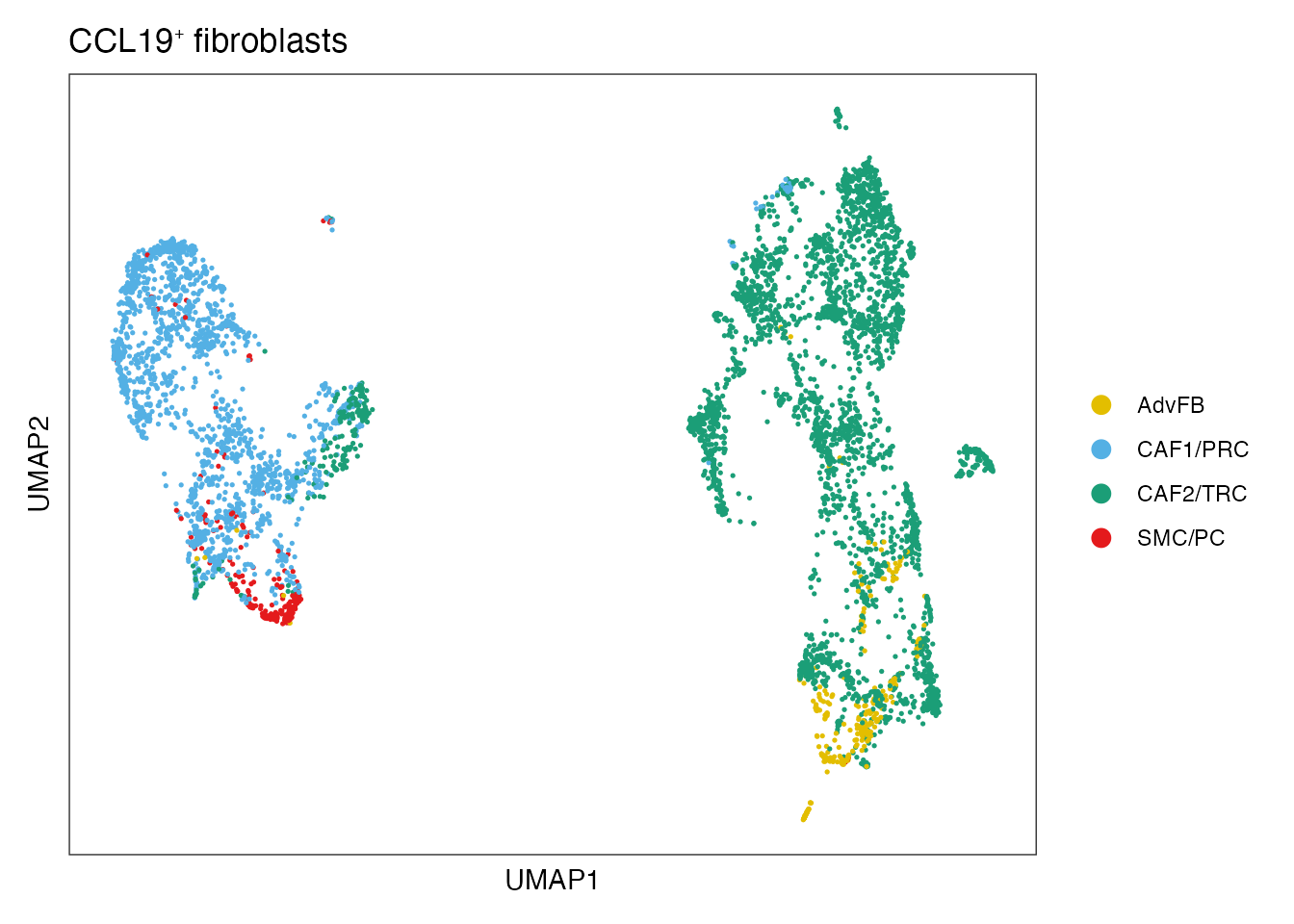
Subset on CCL19⁺ FRCs
NCLS_FRCS <- subset(NSCLC_CCL19_data, cell_type %in% c("CAF2/TRC","CAF1/PRC"))

#Preprocessing
resolution <- c(0.1, 0.25, 0.4, 0.6,0.7, 0.8, 0.9, 1.0, 1.2, 1.4, 1.6, 1.8, 2.0)
NCLS_FRCS <- FindVariableFeatures(NCLS_FRCS, selection.method = "vst", nfeatures = 2000)
NCLS_FRCS <- ScaleData(NCLS_FRCS)
NCLS_FRCS <- RunPCA(object = NCLS_FRCS, npcs = 30, verbose = FALSE,seed.use = 8734)
NCLS_FRCS <- RunTSNE(object = NCLS_FRCS, reduction = "pca", dims = 1:20, seed.use = 8734)
NCLS_FRCS <- RunUMAP(object = NCLS_FRCS, reduction = "pca", dims = 1:20, seed.use = 8734)
NCLS_FRCS <- FindNeighbors(object = NCLS_FRCS, reduction = "pca", dims = 1:20, seed.use = 8734)
for(k in 1:length(resolution)){
  NCLS_FRCS <- FindClusters(object = NCLS_FRCS, resolution = resolution[k], random.seed = 8734)
}
Modularity Optimizer version 1.3.0 by Ludo Waltman and Nees Jan van Eck
Number of nodes: 5023
Number of edges: 172182
Running Louvain algorithm...
Maximum modularity in 10 random starts: 0.9474
Number of communities: 4
Elapsed time: 0 seconds
Modularity Optimizer version 1.3.0 by Ludo Waltman and Nees Jan van Eck
Number of nodes: 5023
Number of edges: 172182
Running Louvain algorithm...
Maximum modularity in 10 random starts: 0.9089
Number of communities: 8
Elapsed time: 0 seconds
Modularity Optimizer version 1.3.0 by Ludo Waltman and Nees Jan van Eck
Number of nodes: 5023
Number of edges: 172182
Running Louvain algorithm...
Maximum modularity in 10 random starts: 0.8838
Number of communities: 9
Elapsed time: 0 seconds
Modularity Optimizer version 1.3.0 by Ludo Waltman and Nees Jan van Eck
Number of nodes: 5023
Number of edges: 172182
Running Louvain algorithm...
Maximum modularity in 10 random starts: 0.8560
Number of communities: 12
Elapsed time: 0 seconds
Modularity Optimizer version 1.3.0 by Ludo Waltman and Nees Jan van Eck
Number of nodes: 5023
Number of edges: 172182
Running Louvain algorithm...
Maximum modularity in 10 random starts: 0.8432
Number of communities: 13
Elapsed time: 0 seconds
Modularity Optimizer version 1.3.0 by Ludo Waltman and Nees Jan van Eck
Number of nodes: 5023
Number of edges: 172182
Running Louvain algorithm...
Maximum modularity in 10 random starts: 0.8315
Number of communities: 15
Elapsed time: 0 seconds
Modularity Optimizer version 1.3.0 by Ludo Waltman and Nees Jan van Eck
Number of nodes: 5023
Number of edges: 172182
Running Louvain algorithm...
Maximum modularity in 10 random starts: 0.8227
Number of communities: 16
Elapsed time: 0 seconds
Modularity Optimizer version 1.3.0 by Ludo Waltman and Nees Jan van Eck
Number of nodes: 5023
Number of edges: 172182
Running Louvain algorithm...
Maximum modularity in 10 random starts: 0.8139
Number of communities: 17
Elapsed time: 0 seconds
Modularity Optimizer version 1.3.0 by Ludo Waltman and Nees Jan van Eck
Number of nodes: 5023
Number of edges: 172182
Running Louvain algorithm...
Maximum modularity in 10 random starts: 0.7990
Number of communities: 17
Elapsed time: 0 seconds
Modularity Optimizer version 1.3.0 by Ludo Waltman and Nees Jan van Eck
Number of nodes: 5023
Number of edges: 172182
Running Louvain algorithm...
Maximum modularity in 10 random starts: 0.7839
Number of communities: 18
Elapsed time: 0 seconds
Modularity Optimizer version 1.3.0 by Ludo Waltman and Nees Jan van Eck
Number of nodes: 5023
Number of edges: 172182
Running Louvain algorithm...
Maximum modularity in 10 random starts: 0.7705
Number of communities: 21
Elapsed time: 0 seconds
Modularity Optimizer version 1.3.0 by Ludo Waltman and Nees Jan van Eck
Number of nodes: 5023
Number of edges: 172182
Running Louvain algorithm...
Maximum modularity in 10 random starts: 0.7591
Number of communities: 22
Elapsed time: 0 seconds
Modularity Optimizer version 1.3.0 by Ludo Waltman and Nees Jan van Eck
Number of nodes: 5023
Number of edges: 172182
Running Louvain algorithm...
Maximum modularity in 10 random starts: 0.7483
Number of communities: 23
Elapsed time: 0 secondsUmap of Re-embedded CCL19⁺ FRC subsets (Figure 4B)
palet_CCL19_FRC <- c("#5050FFFF", "#CE3D32FF")
names(palet_CCL19_FRC) <- c("CAF2/TRC","CAF1/PRC")

DimPlot(NCLS_FRCS, reduction = "umap", group.by = "cell_type",cols = palet_CCL19_FRC)+
  theme_bw() +
  theme(axis.text = element_blank(), axis.ticks = element_blank(),
        panel.grid.minor = element_blank(),
        panel.grid.major = element_blank()) +
  xlab("UMAP1") +
  ylab("UMAP2") + ggtitle(paste0("CCL19", "\U207A ", "Tumor FRCs"))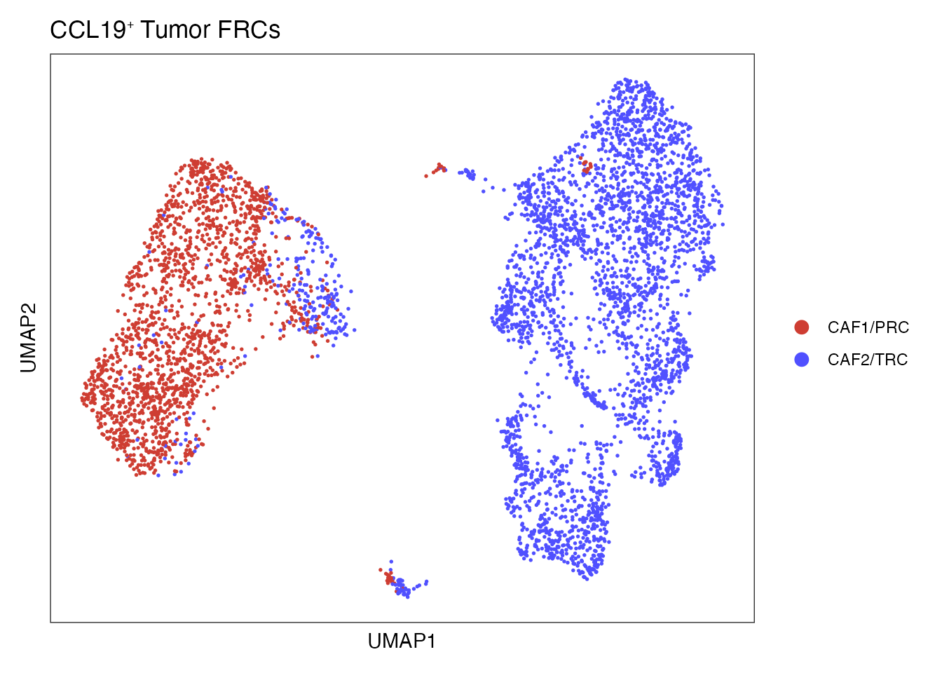
Tonsillar FRC signatures projected on tumor CCL19⁺ FRC subsets (Figure 4C)
Signature SLO-TRC
NSCLC_TRC <-c("CCL19","CCL21","PDPN","ICAM1","VCAM1","LUM","PDGFRA","TNFSF13B")
NSCLC_TRC <- unlist(lapply(NSCLC_TRC, function(x) {
  get_full_gene_name(x,NCLS_FRCS)
}))
slot_type <-"data"
gn <- "Tumor_TRC"
Visualize_GeneSignatures_sc(NCLS_FRCS, NSCLC_TRC, slot_type, 'average.mean',gn) + ggtitle("SLO-TRC signature")
[1] "gene.set.score_Tumor_TRC_data"
Cell names order match in 'mean_expr' and 'object@meta.data':
adding gene set mean expression values in 'object@meta.data$gene.set.score'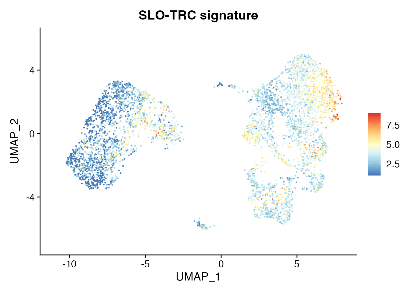
Signature SLO-PRC
NSCLC_PRC <-c("CCL19","CCL21","ITGA1","ITGA7","MCAM","CNN1","NOTCH3","ACTA2","PDGFRB","ANGPT2")
NSCLC_PRC <- unlist(lapply(NSCLC_PRC, function(x) {
  get_full_gene_name(x,NCLS_FRCS)
}))

slot_type <-"data"
gn <- "Tumor_PRC"
Visualize_GeneSignatures_sc(NCLS_FRCS, NSCLC_PRC, slot_type, 'average.mean',gn) + ggtitle("SLO-PRC signature")
[1] "gene.set.score_Tumor_PRC_data"
Cell names order match in 'mean_expr' and 'object@meta.data':
adding gene set mean expression values in 'object@meta.data$gene.set.score'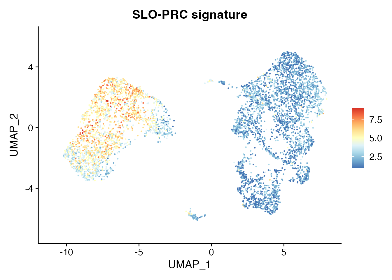
Comparison of transcriptional profiles between NSCLC CCL19⁺ FRCs and Tonsilar FRCs via Multidimensional scaling (MDS)
Read Tonsilar FRC data
Tons_FRC_data <-readRDS(paste0(basedir,"/data/Human/mergedHumanTonsilExtendedDataset_incAcuteTonsilitis_mapped_wocl11+12+14_seuratFRC.rds"))Define color palette
cols<- pal_igv()(51)
names(cols) <- c(0:50)
Tonsilar FRCs
Tons_FRC_data@meta.data$clusterLabel[Tons_FRC_data@meta.data$clusterLabel == "ACTA2+PRC_1"] <- paste0("ACTA2", expression("\U207A"),"PRC_1")
Tons_FRC_data@meta.data$clusterLabel[Tons_FRC_data@meta.data$clusterLabel == "ACTA2+PRC_2"] <- paste0("ACTA2", expression("\U207A"),"PRC_2")
Tons_FRC_data@meta.data$clusterLabel[Tons_FRC_data@meta.data$clusterLabel == "ACTA2+PRC_3"] <- paste0("ACTA2", expression("\U207A"),"PRC_3")
Tons_FRC_data@meta.data$clusterLabel[Tons_FRC_data@meta.data$clusterLabel == "ACTA2+PRC_4"] <- paste0("ACTA2", expression("\U207A"),"PRC_4")
Tons_FRC_data@meta.data$clusterLabel[Tons_FRC_data@meta.data$clusterLabel == "ACTA2+PRC_5"] <- paste0("ACTA2", expression("\U207A"),"PRC_5")
Tons_FRC_data@meta.data$clusterLabel[Tons_FRC_data@meta.data$clusterLabel == "FDC_6"] <- "FDC"
Tons_FRC_data@meta.data$clusterLabel[Tons_FRC_data@meta.data$clusterLabel == "PI16+RC_10"] <- paste0("PI16", expression("\U207A"),"RC_1")
Tons_FRC_data@meta.data$clusterLabel[Tons_FRC_data@meta.data$clusterLabel == "PI16+RC_11"] <- paste0("PI16", expression("\U207A"),"RC_2")
Tons_FRC_data@meta.data$clusterLabel[Tons_FRC_data@meta.data$clusterLabel == "PI16+RC_12"] <- paste0("PI16", expression("\U207A"),"RC_3")
Tons_FRC_data@meta.data$clusterLabel[Tons_FRC_data@meta.data$clusterLabel == "TRC_7"] <- "TRC_1"
Tons_FRC_data@meta.data$clusterLabel[Tons_FRC_data@meta.data$clusterLabel == "TRC_8"] <- "TRC_2"
Tons_FRC_data@meta.data$clusterLabel[Tons_FRC_data@meta.data$clusterLabel == "TRC_9"] <- "TRC_3"

colDataset <- cols[3:15]
names(colDataset) <- unique(Tons_FRC_data$clusterLabel)

DimPlot(Tons_FRC_data, reduction = "umap", group.by = "clusterLabel",cols=colDataset)+
  theme_bw() +
  theme(axis.text = element_blank(), axis.ticks = element_blank(),
        panel.grid.minor = element_blank(),
        panel.grid.major = element_blank()) +
  xlab("UMAP1") +
  ylab("UMAP2") + ggtitle("Tonsilar FRCs (De Martin et al 2023)")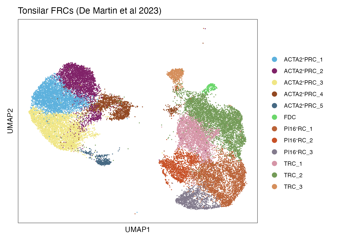
Merge NSCLC TRC and PRC with Tonsilar FRCs
NCLS_FRCS$Disease_short <-rep("NSCLC",nrow(NCLS_FRCS@meta.data))
Tons_FRC_data$Disease_short <-rep("Tonsil",nrow(Tons_FRC_data@meta.data))
colnames(Tons_FRC_data@meta.data)[names(Tons_FRC_data@meta.data) == 'clusterLabel'] <- 'cell_type'

data_merge <- merge(NCLS_FRCS, y = c(Tons_FRC_data),
             add.cell.ids = c("NCLS_FRCS","Tons_FRC_data"),
             project = "merge_nsclc_tonsils")

#Preprocessing
resolution <- c(0.1, 0.25, 0.4, 0.6,0.8, 1.)
data_merge  <- preprocessing(data_merge,resolution)
Modularity Optimizer version 1.3.0 by Ludo Waltman and Nees Jan van Eck
Number of nodes: 33594
Number of edges: 1098322
Running Louvain algorithm...
Maximum modularity in 10 random starts: 0.9641
Number of communities: 6
Elapsed time: 6 seconds
Modularity Optimizer version 1.3.0 by Ludo Waltman and Nees Jan van Eck
Number of nodes: 33594
Number of edges: 1098322
Running Louvain algorithm...
Maximum modularity in 10 random starts: 0.9342
Number of communities: 12
Elapsed time: 7 seconds
Modularity Optimizer version 1.3.0 by Ludo Waltman and Nees Jan van Eck
Number of nodes: 33594
Number of edges: 1098322
Running Louvain algorithm...
Maximum modularity in 10 random starts: 0.9153
Number of communities: 13
Elapsed time: 6 seconds
Modularity Optimizer version 1.3.0 by Ludo Waltman and Nees Jan van Eck
Number of nodes: 33594
Number of edges: 1098322
Running Louvain algorithm...
Maximum modularity in 10 random starts: 0.8977
Number of communities: 17
Elapsed time: 6 seconds
Modularity Optimizer version 1.3.0 by Ludo Waltman and Nees Jan van Eck
Number of nodes: 33594
Number of edges: 1098322
Running Louvain algorithm...
Maximum modularity in 10 random starts: 0.8821
Number of communities: 21
Elapsed time: 5 seconds
Modularity Optimizer version 1.3.0 by Ludo Waltman and Nees Jan van Eck
Number of nodes: 33594
Number of edges: 1098322
Running Louvain algorithm...
Maximum modularity in 10 random starts: 0.8698
Number of communities: 27
Elapsed time: 5 secondsIntegrate data to correct for batch effects due to different tissues via seurat
Step 1
obj.list <-SplitObject(data_merge, split.by = 'cell_type')
#For each object in list we see to run normalization and identify highly variable features
for (i in 1:length(obj.list)){
  #Normalization
  obj.list[[i]] <- NormalizeData(obj.list[[i]], normalization.method = "LogNormalize", scale.factor = 10000)
  #Find high variable genes
  obj.list[[i]] <- FindVariableFeatures(obj.list[[i]], selection.method = "vst", nfeatures = 2000)
}
Step 2
#select features that are repeatedly variable across datasets for integration
features <- SelectIntegrationFeatures(object.list = obj.list)
#Find anchors to integrate the data across different patients (Canonical correlation analysis)
anchors <- FindIntegrationAnchors(object.list = obj.list, anchor.features = features)
# Create an 'integrated' data assay
seurat_integrated <- IntegrateData(anchorset = anchors)
Step 3
# We run a single integrated analysis on all cells!
DefaultAssay(seurat_integrated) <- "integrated"

# Run the standard workflow for visualization and clustering
seurat_integrated <- ScaleData(seurat_integrated, verbose = FALSE)
seurat_integrated <- RunPCA(object = seurat_integrated, npcs = 30, verbose = FALSE,seed.use = 8734)
seurat_integrated <- RunTSNE(object = seurat_integrated, reduction = "pca", dims = 1:20, seed.use = 8734)
seurat_integrated<- RunUMAP(object = seurat_integrated, reduction = "pca", dims = 1:20, seed.use = 8734)
seurat_integrated <- FindNeighbors(object = seurat_integrated, reduction = "pca", dims = 1:20, seed.use = 8734)
#Clustering
resolution <- c(0.1, 0.25, 0.4, 0.6,0.8, 1.,1.2,1.4,1.8)
for(k in 1:length(resolution)){
  seurat_integrated <- FindClusters(object = seurat_integrated, resolution = resolution[k], random.seed = 8734)
}
Apply Divide and conquer MDS algorithm proposed by Delicado P. and C. Pachón-García (2021) for fast MDS computation due to large dataset size
# celltype similarity wth MDS
DefaultAssay(seurat_integrated) <-'integrated'

#Divide-andconquer MDS proposed by Delicado P. and C. Pachón-García (2021)
#MDS computation
mds <- divide_conquer_mds(x = t(GetAssayData(seurat_integrated, slot = 'scale.data')), l = 200, c_points = 5 * 2, r = 2, n_cores = 1)$points
colnames(mds) <- paste0("MDSDIVCONQ_", 1:2)

# Store MDS representation as a custom dimensional reduction field
seurat_integrated[['mds_div_conq']] <- CreateDimReducObject(embeddings = mds, key = 'MDSDIVCONQ_', assay = DefaultAssay(seurat_integrated))

# Save seurat object for later use
#saveRDS(seurat_integrated,paste0(basedir,"/data/Human/Tonsil_Ccl19_TRC_PRC_final_mds_div_conq.rds"))
Multidimensional scaling (MDS) plot
Read integrated object with MDS representation
seurat_integrated <- readRDS(paste0(basedir,"/data/Human/Tonsil_Ccl19_TRC_PRC_final_mds_conq.rds"))Visualize MDS plot (Figure 4D)
mds_tx_condition <- seurat_integrated@reductions$mds_div_conq@cell.embeddings %>%
as.data.frame() %>% cbind(tx = seurat_integrated@meta.data$Disease_short)

mds_tx_celltype <- seurat_integrated@reductions$mds_div_conq@cell.embeddings %>%
as.data.frame() %>% cbind(tx = seurat_integrated@meta.data$cell_type)

mds_tx_TOTAL <- merge(mds_tx_condition, mds_tx_celltype, by=c("MDSDIVCONQ_1", "MDSDIVCONQ_2"), all.x=T, all.y=T)
colnames(mds_tx_TOTAL) <-c("MDS_1", "MDS_2", "Condition","Celltype")

#Color palette
colDataset <- cols[1:15]
names(colDataset) <- unique(seurat_integrated$cell_type)

# Use mean gaussian kernel
mds_tx_TOTAL_gk <- mds_tx_TOTAL %>%
  group_by(Celltype,Condition) %>%
  mutate(count_mds1 = mean(GK(MDS_1))) %>%
  mutate(count_mds2 = mean(GK(MDS_2)))

ggplot(mds_tx_TOTAL_gk, aes(x=count_mds1, y=count_mds2, color=Celltype, shape = Condition)) + geom_point(stroke = 1.5) + ylab("MDS2") + xlab("MDS1") + coord_cartesian(xlim = c(0, max(mds_tx_TOTAL_gk$count_mds1,mds_tx_TOTAL_gk$count_mds2)), ylim = c(0, max(mds_tx_TOTAL_gk$count_mds1,mds_tx_TOTAL_gk$count_mds2)) ) +
scale_color_manual(values=colDataset) + scale_shape_manual(values = c(2, 3)) +
  theme(aspect.ratio = 2,axis.line = element_line(colour = "black"),
    panel.grid.major = element_blank(),
    panel.grid.minor = element_blank(),
    panel.border = element_blank(),
    panel.background = element_blank(),
    axis.text.y = element_text(angle = 0, vjust = 0.5,colour = "black",size = 10),
axis.text.x = element_text(angle = 0, vjust = 0.5,colour = "black",size = 10)) 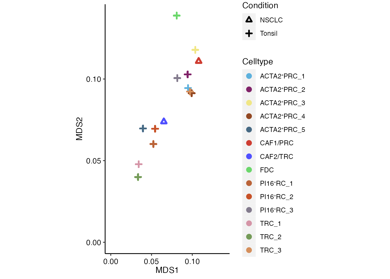
Read NSCLC TIL data
NSCLS_TIL_data <- readRDS(paste0(basedir,"/data/Human/NSCLC_TILs.rds"))Merge NSCLS CCL19⁺ FRCs and NSCLS TILs
same_columns <- intersect(colnames(NSCLS_TIL_data@meta.data),colnames(NCLS_FRCS@meta.data))

NSCLS_TIL_data@meta.data <-NSCLS_TIL_data@meta.data[,same_columns]
NCLS_FRCS@meta.data <-NCLS_FRCS@meta.data[,same_columns]

merged_data<- merge(NSCLS_TIL_data, y = c(NCLS_FRCS),
             add.cell.ids = c('NSCLS_TIL_data','NCLS_FRCS'),
             project = "NSCLC_FRC_TIL")

resolution <- c(0.1, 0.25, 0.4, 0.6, 0.8, 1.,1.2,1.4,1.6,2.)
merged_data  <- preprocessing(merged_data,resolution)
Modularity Optimizer version 1.3.0 by Ludo Waltman and Nees Jan van Eck
Number of nodes: 11699
Number of edges: 402688
Running Louvain algorithm...
Maximum modularity in 10 random starts: 0.9692
Number of communities: 7
Elapsed time: 0 seconds
Modularity Optimizer version 1.3.0 by Ludo Waltman and Nees Jan van Eck
Number of nodes: 11699
Number of edges: 402688
Running Louvain algorithm...
Maximum modularity in 10 random starts: 0.9416
Number of communities: 11
Elapsed time: 1 seconds
Modularity Optimizer version 1.3.0 by Ludo Waltman and Nees Jan van Eck
Number of nodes: 11699
Number of edges: 402688
Running Louvain algorithm...
Maximum modularity in 10 random starts: 0.9236
Number of communities: 13
Elapsed time: 1 seconds
Modularity Optimizer version 1.3.0 by Ludo Waltman and Nees Jan van Eck
Number of nodes: 11699
Number of edges: 402688
Running Louvain algorithm...
Maximum modularity in 10 random starts: 0.9030
Number of communities: 15
Elapsed time: 1 seconds
Modularity Optimizer version 1.3.0 by Ludo Waltman and Nees Jan van Eck
Number of nodes: 11699
Number of edges: 402688
Running Louvain algorithm...
Maximum modularity in 10 random starts: 0.8869
Number of communities: 20
Elapsed time: 1 seconds
Modularity Optimizer version 1.3.0 by Ludo Waltman and Nees Jan van Eck
Number of nodes: 11699
Number of edges: 402688
Running Louvain algorithm...
Maximum modularity in 10 random starts: 0.8738
Number of communities: 21
Elapsed time: 1 seconds
Modularity Optimizer version 1.3.0 by Ludo Waltman and Nees Jan van Eck
Number of nodes: 11699
Number of edges: 402688
Running Louvain algorithm...
Maximum modularity in 10 random starts: 0.8610
Number of communities: 22
Elapsed time: 1 seconds
Modularity Optimizer version 1.3.0 by Ludo Waltman and Nees Jan van Eck
Number of nodes: 11699
Number of edges: 402688
Running Louvain algorithm...
Maximum modularity in 10 random starts: 0.8499
Number of communities: 24
Elapsed time: 1 seconds
Modularity Optimizer version 1.3.0 by Ludo Waltman and Nees Jan van Eck
Number of nodes: 11699
Number of edges: 402688
Running Louvain algorithm...
Maximum modularity in 10 random starts: 0.8399
Number of communities: 28
Elapsed time: 1 seconds
Modularity Optimizer version 1.3.0 by Ludo Waltman and Nees Jan van Eck
Number of nodes: 11699
Number of edges: 402688
Running Louvain algorithm...
Maximum modularity in 10 random starts: 0.8217
Number of communities: 29
Elapsed time: 1 secondsFRC-immune cell interactions in NSCLC via Cellchat (Suoqin Jin et al., 2021)
Convert seurat object to cellchat object
#Define color palet
palet <- c("#5050FFFF", "#CE3D32FF", "#4DAF4A","#FB9A99","#377EB8","#A65628","#222F75")
names(palet) <- c( "CAF2/TRC","CAF1/PRC", paste0("CD4", "\u207A ", "T cells"), paste0("CD8", "\u207A ", "T cells"), "B cells", "Regulatory T cells",paste0("Cycling CD8", "\u207A ", "T cells"))

# Interactome analysis
cellchat <- Cellchat_Analysis(merged_data)
[1] "Create a CellChat object from a data matrix"
Set cell identities for the new CellChat object
The cell groups used for CellChat analysis are B cells CAF1/PRC CAF2/TRC CD4⁺ T cells CD8⁺ T cells Cycling CD8⁺ T cells Regulatory T cells cellchat <-CellChatDownstreamAnalysis(cellchat,"human",thresh = 0.05)triMean is used for calculating the average gene expression per cell group.
[1] ">>> Run CellChat on sc/snRNA-seq data <<< [2025-10-01 17:47:36.645817]"
[1] ">>> CellChat inference is done. Parameter values are stored in `object@options$parameter` <<< [2025-10-01 17:49:04.240146]"Interactome analysis (Figure 4E)
gg <- netAnalysis_signalingRole_scatter(cellchat,color.use = palet)
gg <- gg + ggtitle("Interactome analysis (Cellchat)")
gg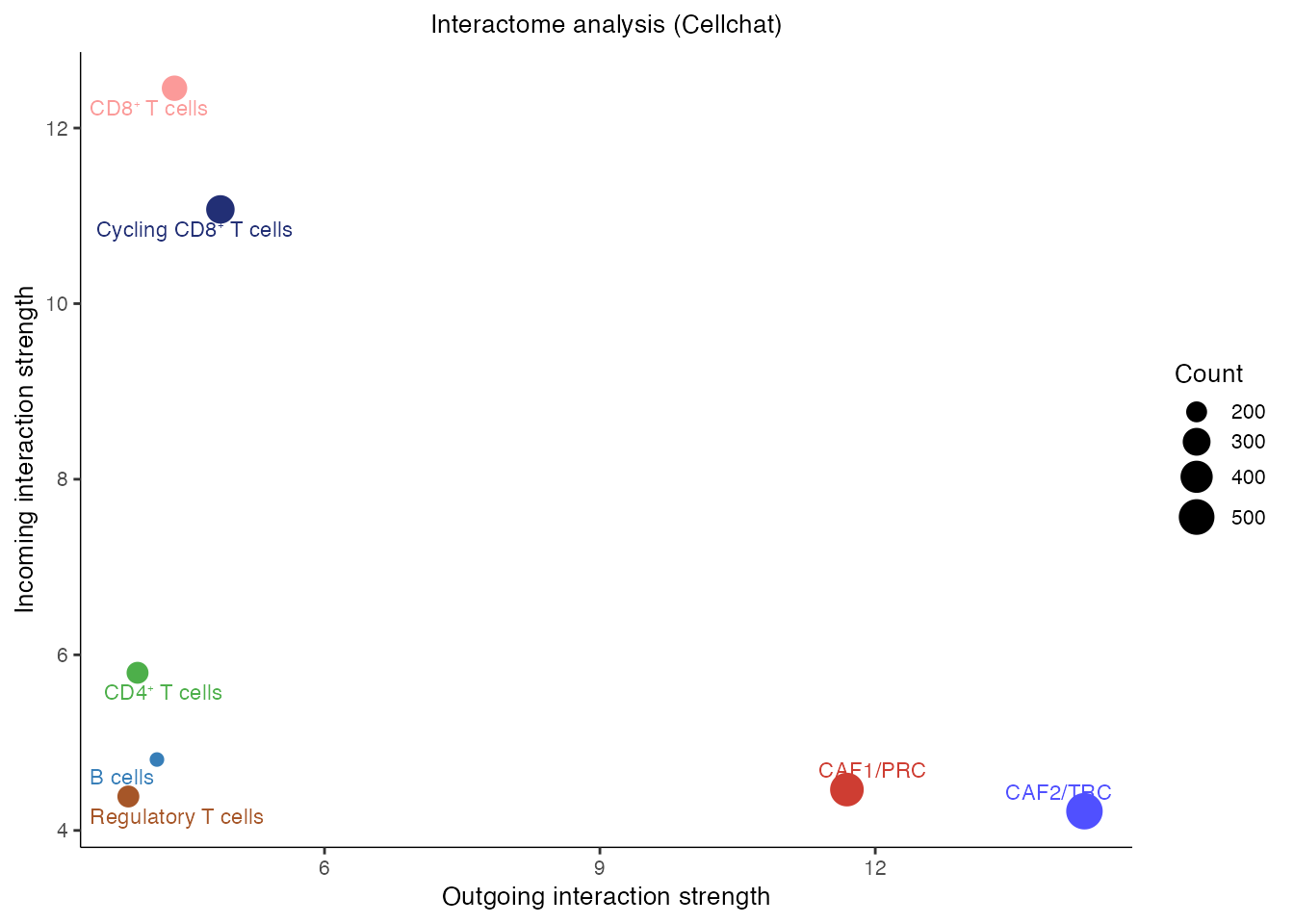 ### Outgoing signaling patterns
selectK(cellchat, pattern = "outgoing")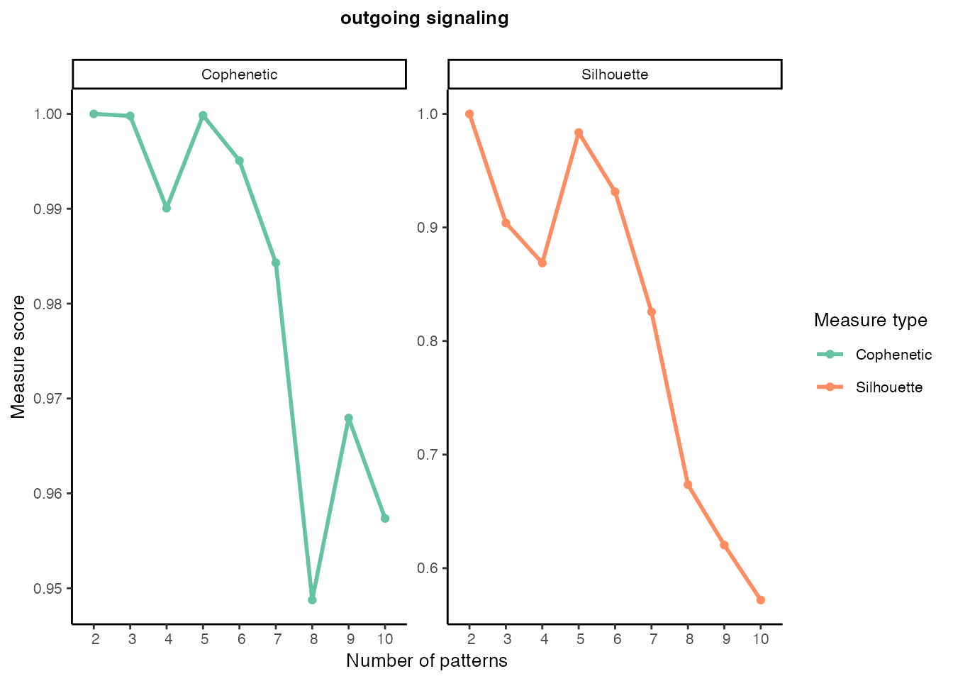
Incoming signaling patterns
selectK(cellchat, pattern = "incoming")
Incoming and outgoing patterns
cellchat <- identifyCommunicationPatterns(cellchat, pattern = "outgoing", k = 5, color.use = palet)
cellchat <- identifyCommunicationPatterns(cellchat, pattern = "incoming", k = 6, color.use = palet)
Joint dotplot for highlighting incoming and outcoming communication patterns explicitly for pathways with active signaling between FRCs and immune cells (Figure 4F)
order_list <-c("CAF2/TRC","CAF1/PRC",
               paste0("CD8", "\u207A ", "T cells"),
               paste0("Cycling CD8", "\u207A ", "T cells"),
               paste0("CD4", "\u207A ", "T cells"),"B cells", "Regulatory T cells")

pathways<- cellchat@netP$pathways

gg <-comAnalysis_joint_dot(cellchat,color.use = palet,font.size = 8,pathways = pathways, order_list = order_list)$gg
shared_signaling <- comAnalysis_joint_dot(cellchat,color.use = palet,font.size = 8,pathways = pathways, order_list = order_list)$new_df_list
gg
Session info
sessionInfo()R version 4.3.1 (2023-06-16)
Platform: aarch64-apple-darwin20 (64-bit)
Running under: macOS 15.6.1
Matrix products: default
BLAS: /Library/Frameworks/R.framework/Versions/4.3-arm64/Resources/lib/libRblas.0.dylib
LAPACK: /Library/Frameworks/R.framework/Versions/4.3-arm64/Resources/lib/libRlapack.dylib; LAPACK version 3.11.0
locale:
[1] en_US.UTF-8/en_US.UTF-8/en_US.UTF-8/C/en_US.UTF-8/en_US.UTF-8
time zone: Europe/Zurich
tzcode source: internal
attached base packages:
[1] parallel stats graphics grDevices utils datasets methods
[8] base
other attached packages:
[1] doParallel_1.0.17 iterators_1.0.14 foreach_1.5.2
[4] bigmds_3.0.0 ggsci_3.0.0 harmony_1.2.0
[7] Rcpp_1.0.11 CellChat_1.6.1 igraph_1.5.0.1
[10] dplyr_1.1.2 NMF_0.26 Biobase_2.60.0
[13] BiocGenerics_0.46.0 cluster_2.1.4 rngtools_1.5.2
[16] registry_0.5-1 dittoSeq_1.12.1 ggplot2_3.4.2
[19] SeuratObject_5.1.0 Seurat_4.3.0.1 purrr_1.0.1
[22] here_1.0.1 magrittr_2.0.3 circlize_0.4.15
[25] tidyr_1.3.0 tibble_3.2.1 workflowr_1.7.1
loaded via a namespace (and not attached):
[1] RcppAnnoy_0.0.21 splines_4.3.1
[3] later_1.3.1 bitops_1.0-7
[5] polyclip_1.10-4 ggnetwork_0.5.12
[7] lifecycle_1.0.3 rstatix_0.7.2
[9] rprojroot_2.0.3 globals_0.16.2
[11] processx_3.8.2 lattice_0.21-8
[13] MASS_7.3-60 backports_1.4.1
[15] plotly_4.10.2 sass_0.4.7
[17] rmarkdown_2.23 jquerylib_0.1.4
[19] yaml_2.3.7 httpuv_1.6.11
[21] sctransform_0.4.1 spam_2.10-0
[23] sp_2.0-0 spatstat.sparse_3.0-2
[25] reticulate_1.36.1 cowplot_1.1.1
[27] pbapply_1.7-2 RColorBrewer_1.1-3
[29] abind_1.4-5 zlibbioc_1.46.0
[31] Rtsne_0.16 GenomicRanges_1.52.0
[33] RCurl_1.98-1.12 pracma_2.4.4
[35] git2r_0.33.0 GenomeInfoDbData_1.2.10
[37] IRanges_2.34.1 S4Vectors_0.38.1
[39] svd_0.5.5 ggrepel_0.9.3
[41] irlba_2.3.5.1 listenv_0.9.0
[43] spatstat.utils_3.1-0 pheatmap_1.0.12
[45] RSpectra_0.16-1 goftest_1.2-3
[47] spatstat.random_3.1-5 fitdistrplus_1.1-11
[49] parallelly_1.36.0 svglite_2.1.1
[51] leiden_0.4.3 codetools_0.2-19
[53] DelayedArray_0.28.0 tidyselect_1.2.0
[55] shape_1.4.6 farver_2.1.1
[57] matrixStats_1.0.0 stats4_4.3.1
[59] spatstat.explore_3.2-1 jsonlite_1.8.7
[61] GetoptLong_1.0.5 BiocNeighbors_1.18.0
[63] ellipsis_0.3.2 progressr_0.13.0
[65] ggalluvial_0.12.5 ggridges_0.5.4
[67] survival_3.5-5 systemfonts_1.0.4
[69] tools_4.3.1 ragg_1.2.5
[71] sna_2.7-1 ica_1.0-3
[73] glue_1.6.2 gridExtra_2.3
[75] SparseArray_1.2.4 xfun_0.39
[77] MatrixGenerics_1.12.3 GenomeInfoDb_1.36.1
[79] withr_2.5.0 BiocManager_1.30.21.1
[81] fastmap_1.1.1 fansi_1.0.4
[83] callr_3.7.3 digest_0.6.33
[85] R6_2.5.1 mime_0.12
[87] textshaping_0.3.6 colorspace_2.1-0
[89] Cairo_1.6-1 scattermore_1.2
[91] tensor_1.5 spatstat.data_3.0-1
[93] utf8_1.2.3 generics_0.1.3
[95] data.table_1.14.8 FNN_1.1.3.2
[97] httr_1.4.6 htmlwidgets_1.6.2
[99] S4Arrays_1.2.1 whisker_0.4.1
[101] uwot_0.1.16 pkgconfig_2.0.3
[103] gtable_0.3.3 ComplexHeatmap_2.16.0
[105] lmtest_0.9-40 SingleCellExperiment_1.22.0
[107] XVector_0.40.0 htmltools_0.5.5
[109] carData_3.0-5 dotCall64_1.1-1
[111] clue_0.3-64 scales_1.2.1
[113] png_0.1-8 knitr_1.43
[115] rstudioapi_0.15.0 rjson_0.2.21
[117] reshape2_1.4.4 coda_0.19-4
[119] statnet.common_4.9.0 nlme_3.1-162
[121] cachem_1.0.8 zoo_1.8-12
[123] GlobalOptions_0.1.2 stringr_1.5.0
[125] KernSmooth_2.23-22 miniUI_0.1.1.1
[127] pillar_1.9.0 grid_4.3.1
[129] vctrs_0.6.3 RANN_2.6.1
[131] ggpubr_0.6.0 promises_1.2.0.1
[133] car_3.1-2 xtable_1.8-4
[135] evaluate_0.21 cli_3.6.1
[137] compiler_4.3.1 rlang_1.1.1
[139] crayon_1.5.2 ggsignif_0.6.4
[141] future.apply_1.11.0 labeling_0.4.2
[143] ps_1.7.5 forcats_1.0.0
[145] getPass_0.2-4 plyr_1.8.8
[147] fs_1.6.3 stringi_1.7.12
[149] network_1.18.1 BiocParallel_1.34.2
[151] viridisLite_0.4.2 deldir_1.0-9
[153] gridBase_0.4-7 munsell_0.5.0
[155] lazyeval_0.2.2 spatstat.geom_3.2-4
[157] Matrix_1.6-4 patchwork_1.1.2
[159] future_1.33.0 shiny_1.7.4.1
[161] highr_0.10 SummarizedExperiment_1.30.2
[163] ROCR_1.0-11 broom_1.0.5
[165] bslib_0.5.0 date()[1] "Wed Oct 1 17:52:45 2025"
sessionInfo()R version 4.3.1 (2023-06-16)
Platform: aarch64-apple-darwin20 (64-bit)
Running under: macOS 15.6.1
Matrix products: default
BLAS: /Library/Frameworks/R.framework/Versions/4.3-arm64/Resources/lib/libRblas.0.dylib
LAPACK: /Library/Frameworks/R.framework/Versions/4.3-arm64/Resources/lib/libRlapack.dylib; LAPACK version 3.11.0
locale:
[1] en_US.UTF-8/en_US.UTF-8/en_US.UTF-8/C/en_US.UTF-8/en_US.UTF-8
time zone: Europe/Zurich
tzcode source: internal
attached base packages:
[1] parallel stats graphics grDevices utils datasets methods
[8] base
other attached packages:
[1] doParallel_1.0.17 iterators_1.0.14 foreach_1.5.2
[4] bigmds_3.0.0 ggsci_3.0.0 harmony_1.2.0
[7] Rcpp_1.0.11 CellChat_1.6.1 igraph_1.5.0.1
[10] dplyr_1.1.2 NMF_0.26 Biobase_2.60.0
[13] BiocGenerics_0.46.0 cluster_2.1.4 rngtools_1.5.2
[16] registry_0.5-1 dittoSeq_1.12.1 ggplot2_3.4.2
[19] SeuratObject_5.1.0 Seurat_4.3.0.1 purrr_1.0.1
[22] here_1.0.1 magrittr_2.0.3 circlize_0.4.15
[25] tidyr_1.3.0 tibble_3.2.1 workflowr_1.7.1
loaded via a namespace (and not attached):
[1] RcppAnnoy_0.0.21 splines_4.3.1
[3] later_1.3.1 bitops_1.0-7
[5] polyclip_1.10-4 ggnetwork_0.5.12
[7] lifecycle_1.0.3 rstatix_0.7.2
[9] rprojroot_2.0.3 globals_0.16.2
[11] processx_3.8.2 lattice_0.21-8
[13] MASS_7.3-60 backports_1.4.1
[15] plotly_4.10.2 sass_0.4.7
[17] rmarkdown_2.23 jquerylib_0.1.4
[19] yaml_2.3.7 httpuv_1.6.11
[21] sctransform_0.4.1 spam_2.10-0
[23] sp_2.0-0 spatstat.sparse_3.0-2
[25] reticulate_1.36.1 cowplot_1.1.1
[27] pbapply_1.7-2 RColorBrewer_1.1-3
[29] abind_1.4-5 zlibbioc_1.46.0
[31] Rtsne_0.16 GenomicRanges_1.52.0
[33] RCurl_1.98-1.12 pracma_2.4.4
[35] git2r_0.33.0 GenomeInfoDbData_1.2.10
[37] IRanges_2.34.1 S4Vectors_0.38.1
[39] svd_0.5.5 ggrepel_0.9.3
[41] irlba_2.3.5.1 listenv_0.9.0
[43] spatstat.utils_3.1-0 pheatmap_1.0.12
[45] RSpectra_0.16-1 goftest_1.2-3
[47] spatstat.random_3.1-5 fitdistrplus_1.1-11
[49] parallelly_1.36.0 svglite_2.1.1
[51] leiden_0.4.3 codetools_0.2-19
[53] DelayedArray_0.28.0 tidyselect_1.2.0
[55] shape_1.4.6 farver_2.1.1
[57] matrixStats_1.0.0 stats4_4.3.1
[59] spatstat.explore_3.2-1 jsonlite_1.8.7
[61] GetoptLong_1.0.5 BiocNeighbors_1.18.0
[63] ellipsis_0.3.2 progressr_0.13.0
[65] ggalluvial_0.12.5 ggridges_0.5.4
[67] survival_3.5-5 systemfonts_1.0.4
[69] tools_4.3.1 ragg_1.2.5
[71] sna_2.7-1 ica_1.0-3
[73] glue_1.6.2 gridExtra_2.3
[75] SparseArray_1.2.4 xfun_0.39
[77] MatrixGenerics_1.12.3 GenomeInfoDb_1.36.1
[79] withr_2.5.0 BiocManager_1.30.21.1
[81] fastmap_1.1.1 fansi_1.0.4
[83] callr_3.7.3 digest_0.6.33
[85] R6_2.5.1 mime_0.12
[87] textshaping_0.3.6 colorspace_2.1-0
[89] Cairo_1.6-1 scattermore_1.2
[91] tensor_1.5 spatstat.data_3.0-1
[93] utf8_1.2.3 generics_0.1.3
[95] data.table_1.14.8 FNN_1.1.3.2
[97] httr_1.4.6 htmlwidgets_1.6.2
[99] S4Arrays_1.2.1 whisker_0.4.1
[101] uwot_0.1.16 pkgconfig_2.0.3
[103] gtable_0.3.3 ComplexHeatmap_2.16.0
[105] lmtest_0.9-40 SingleCellExperiment_1.22.0
[107] XVector_0.40.0 htmltools_0.5.5
[109] carData_3.0-5 dotCall64_1.1-1
[111] clue_0.3-64 scales_1.2.1
[113] png_0.1-8 knitr_1.43
[115] rstudioapi_0.15.0 rjson_0.2.21
[117] reshape2_1.4.4 coda_0.19-4
[119] statnet.common_4.9.0 nlme_3.1-162
[121] cachem_1.0.8 zoo_1.8-12
[123] GlobalOptions_0.1.2 stringr_1.5.0
[125] KernSmooth_2.23-22 miniUI_0.1.1.1
[127] pillar_1.9.0 grid_4.3.1
[129] vctrs_0.6.3 RANN_2.6.1
[131] ggpubr_0.6.0 promises_1.2.0.1
[133] car_3.1-2 xtable_1.8-4
[135] evaluate_0.21 cli_3.6.1
[137] compiler_4.3.1 rlang_1.1.1
[139] crayon_1.5.2 ggsignif_0.6.4
[141] future.apply_1.11.0 labeling_0.4.2
[143] ps_1.7.5 forcats_1.0.0
[145] getPass_0.2-4 plyr_1.8.8
[147] fs_1.6.3 stringi_1.7.12
[149] network_1.18.1 BiocParallel_1.34.2
[151] viridisLite_0.4.2 deldir_1.0-9
[153] gridBase_0.4-7 munsell_0.5.0
[155] lazyeval_0.2.2 spatstat.geom_3.2-4
[157] Matrix_1.6-4 patchwork_1.1.2
[159] future_1.33.0 shiny_1.7.4.1
[161] highr_0.10 SummarizedExperiment_1.30.2
[163] ROCR_1.0-11 broom_1.0.5
[165] bslib_0.5.0